
Conas colúin agus sraitheanna a thrasuí / a thiontú ina gcolún aonair?
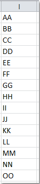
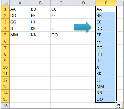
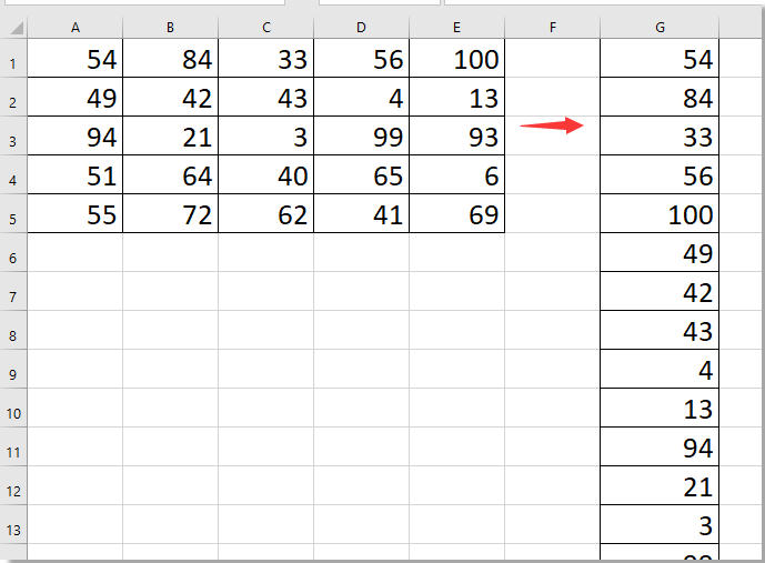
Nuair a úsáideann tú Excel bileog oibre, uaireanta, comhlíonfaidh tú an fhadhb seo: conas a d'fhéadfá raon sonraí a thiontú nó a thrasuí i gcolún amháin? (Féach na screenshots seo a leanas:) Anois, tugaim isteach trí chleas tapaidh duit chun an fhadhb seo a réiteach.

Colúin agus sraitheanna a thrasuí / a thiontú ina gcolún aonair le foirmle

Colúin agus sraitheanna a thrasuí / a thiontú ina gcolún aonair le cód VBA

Trasurigh/Tiontaigh colúin agus sraitheanna i gcolún singil le Kutools for Excelsmaoineamh maith3


Colúin agus sraitheanna a thrasuí / a thiontú ina gcolún aonair le foirmle

Is féidir leis an bhfoirmle fhada seo a leanas cabhrú leat raon sonraí a thrasuí go tapa i gcolún, déan é seo le do thoil:

1. Ar dtús, sainmhínigh ainm raon do do raon sonraí, roghnaigh na sonraí raon a theastaíonn uait a thiontú, cliceáil ar dheis agus roghnaigh Sainmhínigh Ainm foirm an roghchlár comhthéacs. Sa Ainm Nua bosca dialóige, iontráil ainm an raoin atá uait. Ansin cliceáil OK. Féach an pictiúr:

2. Tar éis ainm an raoin a shonrú, ansin cliceáil cill bán, sa sampla seo, cliceáilfidh mé cill E1, agus ansin cuirfidh mé an fhoirmle seo isteach: =INDEX(MyData,1+INT((ROW(A1)-1)/COLUMNS(MyData)),MOD(ROW(A1)-1+COLUMNS(MyData),COLUMNS(MyData))+1).

nótaí: MySonraí is é ainm raon na sonraí roghnaithe, is féidir leat iad a athrú de réir mar is gá duit.

3. Ansin tarraing an fhoirmle síos go dtí an cill go dtí go dtaispeánfar an fhaisnéis earráide. Aistríodh na sonraí go léir sa raon i gcolún amháin. Féach an pictiúr:


Trasuigh raon go tapa go colún/as a chéile/ nó vice versa i Excel

I gcásanna áirithe, b'fhéidir go mbeidh ort raon cealla a thrasuí i gcolún amháin nó i ndiaidh a chéile, nó vice versa, colún nó ró a thiontú ina sraitheanna agus colúin iolracha i Excel leathán. An bhfuil aon bhealach tapa agat chun é a réiteach? Seo an Raon Trasuí feidhm i Kutools for Excel in ann gach post thuas a láimhseáil go héasca.Cliceáil le haghaidh triail lán-feiceáil saor in aisce i 30 laethanta!
doc1
 
Kutools for Excel: le níos mó ná 300 handy Excel breiseáin, saor in aisce chun iarracht a dhéanamh gan aon teorainn i 30 lá.

Colúin agus sraitheanna a thrasuí / a thiontú ina gcolún aonair le cód VBA

Leis an gcód VBA seo a leanas, is féidir leat na colúin agus na sraitheanna iolracha a cheangal le chéile i gcolún amháin.

1. Coinnigh síos an ALT + F11 eochracha a oscailt Microsoft Visual Basic d’Fheidhmchláir fhuinneog.

2. cliceáil Ionsáigh > Modúil, agus greamaigh an cód seo a leanas sa Modúil fhuinneog.

Sub ConvertRangeToColumn()
'Updateby20131126
Dim Range1 As Range, Range2 As Range, Rng As Range
Dim rowIndex As Integer
xTitleId = "KutoolsforExcel"
Set Range1 = Application.Selection
Set Range1 = Application.InputBox("Source Ranges:", xTitleId, Range1.Address, Type:=8)
Set Range2 = Application.InputBox("Convert to (single cell):", xTitleId, Type:=8)
rowIndex = 0
Application.ScreenUpdating = False
For Each Rng In Range1.Rows
    Rng.Copy
    Range2.Offset(rowIndex, 0).PasteSpecial Paste:=xlPasteAll, Transpose:=True
    rowIndex = rowIndex + Rng.Columns.Count
Next
Application.CutCopyMode = False
Application.ScreenUpdating = True
End Sub

3. Brúigh F5 eochair chun an cód a rith, agus taispeántar dialóg duit raon a roghnú le tiontú. Féach an pictiúr:

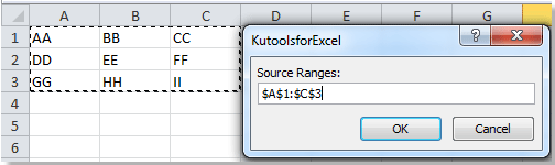
4. Ansin cliceáil Ok, agus taispeántar dialóg eile chun cill singil a roghnú chun an toradh a chur amach, féach an scáileán:

5. Agus cliceáil Ok, ansin athraítear ábhar cille an raoin go liosta de cholún, féach an scáileán:

doc-convert-range-range-to-column11


Trasurigh/Tiontaigh colúin agus sraitheanna i gcolún singil le Kutools for Excel

B’fhéidir go bhfuil an fhoirmle ró-fhada le cuimhneamh agus go bhfuil teorainn éigin ag an gcód VBA leat, sa chás seo, ná bíodh imní ort, anseo tabharfaidh mé uirlis níos éasca agus níos ilfheidhme isteach duit-Kutools for Excel, Lena Transform Range fóntais, agus is féidir leat an fhadhb seo a réiteach go tapa agus go háisiúil.

Kutools for Excel, le níos mó ná 300 feidhmeanna úsáideacha, déanann sé do phoist níos éasca. 

Tar éis suiteáil saor in aisce Kutools for Excel, déan mar atá thíos le do thoil:

1. Roghnaigh an raon is mian leat a thrasuí.

2. cliceáil Kutools > Transform Range, féach ar an scáileán:

raon tiontaithe doc go colún 12

3. Sa Transform Range dialóg, roghnaigh Range to single column rogha, féach an scáileán:

raon tiontaithe doc go colún 13

4. Ansin cliceáil OK, agus sonraigh cill chun an toradh ón mbosca pop-amach a chur.

raon tiontaithe doc go colún 14

5. cliceáil OK, agus rinneadh na sonraí iolracha colún agus sraitheanna a thrasuí i gcolún amháin.
raon tiontaithe doc go colún 15

Más mian leat colún a thiontú go raon le sraitheanna seasta, is féidir leat an Transform Range feidhm chun é a láimhseáil go tapa.
raon tiontaithe doc go colún 16


Trasnaigh an traschlár go dtí an tábla a liostú leis Kutools for Excel

Má tá tras-tábla agat is gá a thiontú go tábla liosta mar a thaispeántar thíos ar an scáileán, ach na sonraí a athsheiceáil ceann ar cheann, is féidir leat iad a úsáid freisin Kutools for Excel'S Transpose Table Dimensions fóntais a thiontú go tapa idir tras tábla agus liosta i Excel.
raon tiontaithe doc go colún 19

Tar éis suiteáil saor in aisce Kutools for Excel, déan mar atá thíos le do thoil:

1. Roghnaigh an tras-tábla a theastaíonn uait a thiontú go liosta, cliceáil Kutools > Range > Transpose Table Dimensions.
raon tiontaithe doc go colún 18

2. I Transpose Table Dimension dialóg, seiceáil Cross table to list rogha ar Transpose type alt, roghnaigh cill chun an tábla formáide nua a chur.
raon tiontaithe doc go colún 18

3. cliceáil Ok, anois tá an tras-tábla tiontaithe go liosta.


Earraí gaolmhara:

Conas a chéile a athrú go colún i Excel?

Conas colún amháin a thrasuíomh / a thiontú go colúin iolracha i Excel?

Conas colúin agus sraitheanna a thrasuí / a thiontú ina ndiaidh a chéile?

Uirlisí Táirgiúlachta Oifige is Fearr

Oifig Tacaíochta/Excel 2007-2021 agus 365 | Ar fáil i 44 Teanga | Éasca le Díshuiteáil go hiomlán

Gnéithe Coitianta: Aimsigh/Aibhsigh/Aithnigh Dúblaigh   |  Scrios Sraitheanna Bána   |  Comhcheangail Colúin nó Cealla gan Sonraí a Chailleadh   |   Babhta gan Foirmle ...
Cuardaigh Super: Ilchritéir VLookup    VLookup Illuachanna  |   VLookup Trasna Ilbhileoga   |   Amharc doiléir ....
Liosta anuas Casta: Go tapa Cruthaigh Liosta Anuas   |  Liosta anuas Cleithiúnach   |  Liosta Buail Isteach Ilroghnacha ....
Bainisteoir Colún: Cuir Líon Sonrach Colún leis  |  Colúin Bog  |  Scoránaigh Stádas Infheictheachta na gColún Ceilte  |  Déan comparáid idir Raonta & Colúin ...
Gnéithe Réadmhaoin: Fócas Eangaí   |  Amharc Dearaidh   |   Barra Mór na Foirmle    Leabhar Oibre & Bainisteoir Bileog   |  Leabharlann Acmhainní (Uaththéacs)   |  Piocálaí Dáta   |  Comhcheangail Bileoga Oibre   |  Criptigh/Díchriptigh Cealla    Seol Ríomhphost trí Liosta   |  Scagaire Super   |   Scagaire Speisialta (scagaire trom/iodálach/stailc tríd...) ...
Barr 15 Uirlisí12 Téacs uirlisí (Cuir Téacs, Bain Carachtair,...)   |   50 + Cairt cineálacha (Cairt Gantt,...)   |   40+ Praiticiúil Foirmlí (Ríomh aois bunaithe ar lá breithe,...)   |   19 Insertion uirlisí (Cuir isteach Cód QR, Ionsáigh Pictiúr ón gCosán,...)   |   12 Tiontú uirlisí (Uimhreacha go Words, Comhshó Airgeadra,...)   |   7 Cumaisc & Scoilt uirlisí (Sraitheanna Comhcheangail Casta, Cealla Scoilt,...)   |   ... agus eile

Kutools for Excel Tá breis is 300 gné ann, A chinntiú nach bhfuil uait ach cliceáil ar shiúl...

Supercharge Do Excel scileanna: Éifeachtúlacht Taithí Mar Riamh Roimhe Le Kutools for Excel  (Triail Iomlán 30-Lá Saor in Aisce)

cluaisín kte 201905

Ráthaíocht Neamhchoinníollach Airgid Ar Ais 60-LáLeigh Nios mo... Íoslódáil saor in aisce ... Ceannach ... 

Office Tab Tugann sé comhéadan Tabbed chuig Oifig, agus Déan do chuid Oibre i bhfad níos éasca

  • Cumasaigh eagarthóireacht agus léamh tabáilte isteach Word, Excel, Pointe cumhachta, Foilsitheoir, Rochtain, Visio agus Tionscadal.
  • Oscail agus cruthaigh cáipéisí iolracha i gcluaisíní nua den fhuinneog chéanna, seachas i bhfuinneoga nua.
  • Méaduithe ar do tháirgiúlacht faoi 50%, agus laghdaítear na céadta cad a tharlaíonn nuair luiche duit gach lá! (Triail Iomlán 30-Lá Saor in Aisce)
Ráthaíocht Neamhchoinníollach Airgid Ar Ais 60-LáLeigh Nios mo... Íoslódáil saor in aisce ... Ceannach ... 
 
Comments (58)
No ratings yet. Be the first to rate!
This comment was minimized by the moderator on the site
thanks for the tutor, very helpfull
This comment was minimized by the moderator on the site
Wow! This is amazing! My data starts on A2 rather than A1 but when I change that in the formula it's grabbing B2 to start rather than A2. I've tried changing things up but can't seem to get it to work. Can you please LMK what I need to change in the formula? Thanks in advance and appreciate any advise!
This comment was minimized by the moderator on the site
Hello, Graves
Yes, as you said, the formula is not correct when the data starts from A2, in this case, you can apply the following formula:
=OFFSET(mydata,TRUNC((ROW()-ROW($G$1))/COLUMNS(mydata)),MOD(ROW()-ROW($G$1),COLUMNS(mydata)),1,1)

Note: In the above fromula, mydata is the range name of the selected data, G1 is the cell you enter this formula, please change them to your own.
Please have a try, hope it can help you!
This comment was minimized by the moderator on the site
Convert table to one column, ignore blank cell and duplicates value. How ?
This comment was minimized by the moderator on the site
After converting the table to a column, using Excel' Remove Duplicate feature to remove the duplicates, then select the column range, use the Delete Blank Rows of Kutools for Excel to remove the blank cells.
This comment was minimized by the moderator on the site
Thank you so much! :)
This comment was minimized by the moderator on the site
the data i am transposing to single column from rows have blanks in it how can i ignore them while transposing
This comment was minimized by the moderator on the site
Hi, sai, you can transpose them to single column firstly, then remove the blank rows. How to remove blank rows, you can go to this article, it introduces 4 ways to remove blank rows, there must be one method can help you. https://www.extendoffice.com/documents/excel/525-excel-remove-blank-rows.html
This comment was minimized by the moderator on the site
thanks a lot; beautifull :-)
This comment was minimized by the moderator on the site
Worked like a charm. Thanks a lot
This comment was minimized by the moderator on the site
thanxs you have reduced my too much time....wonderful
This comment was minimized by the moderator on the site
What if the table you start with has a range of values that is different for each row? Example: Say the table doesn't have FF, KK and LL, how do you make a single column from that table without doing them above example by hand?
This comment was minimized by the moderator on the site
Just try above methods, if they cannot work, please tell me and upload your data as a picture to give some details
This comment was minimized by the moderator on the site
THAT'S AMAZING! THANKYOU
This comment was minimized by the moderator on the site
Hi Friend I/m also facing a problem in excel

My data are column-wise

3.26mm 3.05mm 3.10mm
0.1285 0.1200 0.1220
1/4 1/4 6mm
1-1/8 1-1/8 28mm
2-5/8 2-5/8 66mm


I want to arrange all in a single column

3.05mm
0.1200
1/4
1-1/8
2-5/8
3.10mm
0.1220
6mm
28mm
66mm


Kindly share me formula or valuable suggestion. It's urgent for me. Please help me on priority bases.
This comment was minimized by the moderator on the site
HI,
This formula is not working for me. giving error.
here is my data

1 A
2 B
3 C
4 D
5 E
6 F
7 G
8 H
9 I
10 J
This needs to be converted to the below

1
2
A
B
3
4
C
D
5
6
E
F
7
8
G
H
9
10
I
J


PLEASE HELP ME ASAP. ITS REALLY URGENT. THANK YOU
This comment was minimized by the moderator on the site
I want to convert multiple column into single row in sequene. for example
jan feb march april may june

I want in this way

jan

feb

march

april

may

please comment
This comment was minimized by the moderator on the site
Copy the data into memory, then use the Paste Special, Tranpose option, this will convert your row of data into a column of data.
This comment was minimized by the moderator on the site
This did not work for me because I have 98 columns and 230 rows of uneven data. That is ROW 1 may have only 3 entries (A1, B1 & C1). While, row 2 may have 5 entries (A1, B1, C1, D1, E1) etc....etc..... you get the gist over the huge table of 98 columns and 230 rows.


The formula did not work. Any suggestions?
This comment was minimized by the moderator on the site
Hi. . . I have multiple range with same dimension in each sheet of excel file.
Is it possible to transform column row range into single column for each sheet all at once?
This comment was minimized by the moderator on the site
Hello all, Is there a way to transpose multiple columns into single column based on a primary key, without using kutools? Example: Left table should be converted into right table: Id A B C D ID Category 1 0 3 1 0 1 B 2 1 2 1 0 1 B 3 0 0 1 2 1 B 4 0 1 0 0 1 C 5 2 0 0 1 2 A 2 B 2 B 2 C 3 C 3 D 3 D 4 B 5 A 5 A 5 D
This comment was minimized by the moderator on the site
To get from A1 B1 C1 A2 B2 C2 to A1 A2 B1 B2 C1 C2 Use: =INDEX(Range,MOD(ROW(A1)+ROWS(Range)+1,ROWS(Range)+1),1+INT(ROW(A1)/(ROWS(Range)+1))) Ric
This comment was minimized by the moderator on the site
This formula is not working for me. giving error.
here is my data

A1 B1
A2 B2
A3 B3
A4 B4
A5 B5
A6 B6

This needs to be converted to the below

A1
A2
A3
A4
A5
A6
B1
B2
B3
B4
B5
B6


Please help me
This comment was minimized by the moderator on the site
Using formula with same data ends up showing AA in E1. Not sure why? =INDEX(MyData,1+INT((ROW(A1)-1)/COLUMNS(MyData)),MOD(ROW(A1)-1+COLUMNS(MyData),COLUMNS(MyData))+1)
This comment was minimized by the moderator on the site
Awesome makro! I just have a "minor" problem. I get stuck with an error: "Overflow (Error 6)". I have a table with many empty cells but still 51 columns and 1561 rows. Did anybody already faced such dimensions and problems? I guess it's really just a technical limit that I'm breaching here. Thanks for any help BR Fritz
This comment was minimized by the moderator on the site
Hey, I was wondering how to change the to use two absolute values for the cells. This script is great and I want to add it into a bigger macro that requires no user input. Set Range1 = Application.InputBox("Source Ranges:", xTitleId, Range1.Address, Type:=8) Set Range2 = Application.InputBox("Convert to (single cell):", xTitleId, Type:=8) These two ranges need to be changed, but having some trouble. I tried this but am getting overflow errors. Set Range1 = Range("O2:BA1000") Set Range2 = Range("N2") Any ideas?
This comment was minimized by the moderator on the site
Fantastic VBA for transforming columns and rows into a single sorted column. Just saved me a ton of time. Thanks!
This comment was minimized by the moderator on the site
Amazing.. thanks a ton..
This comment was minimized by the moderator on the site
I have different rows and column with large data. example as Mon jan Feb Cat N S W E N S W E A 4 6 7 8 1 2 3 4 B 1 2 3 4 4 3 2 1 C 3 2 4 4 3 2 4 6 Now i have 2 years data which needs to copy pasted. can we do it any formula to get the February month data under January month.
This comment was minimized by the moderator on the site
Thank you so much. Awesome job!
This comment was minimized by the moderator on the site
Thank you so much!! This saved me so much time and worked perfectly for combining multiple columns into a single column.
This comment was minimized by the moderator on the site
Anyone know how to convert the following: Keeping 1st 3 columns the same but moving the rest of the columns to one column with the data lined up with the correct row. FROM THIS- 14.05.2016 14:35:02 c8k000001 CHO2A ALB2 SI-I LDL_C GLUC3 14.05.2016 14:35:03 c8k000002 CDC05 CHO2A ALB2 SI-I LDL_C 14.05.2016 14:18:15 c8k000003 CDC05 ALTL CHO2A ALB2 SI-I TO THIS - 14.05.2016 14:35:02 c8k000001 CHO2A ALB2 SI-I LDL_C GLUC3 14.05.2016 14:35:03 c8k000002 CDC05 CHO2A ALB2 SI-I LDL_C 14.05.2016 14:18:15 c8k000003 CDC05 ALTL CHO2A ALB2 SI-I Really looking forward to some help with this one. Thanks!
This comment was minimized by the moderator on the site
I need the same solution as Ann. Your help is much appreciated
This comment was minimized by the moderator on the site
If you do this and you also have dates in column A and customers in column (B1;D1), how do you adjus these likewise, so you will get it in column D and E next to the values? This also means that you get one customer and one date 3 times afer each other (18/07/2016) AA (18/07/2016) BB etc.
This comment was minimized by the moderator on the site
In case column A defines the group, and the other cells are exactly like this. You still want to get everything in one cell (except column A) and you want to adjust cell A so it still continues displaying to which value the columns belong after this (which means for example that group 1 has to repeated 3 times. I hope it's clear, can anyone tell me how to do that please
This comment was minimized by the moderator on the site
Transpose/Convert columns and rows into single column with VBA code: THIS WAS AWESOME!!!!!! I was able to merge some columns appropriately and preserve the cell formatting!!!! I have mixed formats within cells (italics, bold, regular etc.) using mostly text relating to species biological analyses, and trying to keep that formatting in excel to use for exports can be VERY difficult when merging or rearranging data. This worked flawlessly and quickly, I kept crashing my VBA for merging cells and preserving formatting because the amount of data within a cell got to be too much. THANK YOU to whoever put this out there!!! Best Wishes, Happy Data Girl
This comment was minimized by the moderator on the site
phewwwwww!!!!! after hours of researching on how to do this GREAT WORK and thanks a lot Kind regards Nathan
This comment was minimized by the moderator on the site
Thanks it was very much helpful.....
This comment was minimized by the moderator on the site
This formula works better when data is in square format, =INDEX(Range,MOD(ROW(B5)-1+COLUMNS(Range),COLUMNS(Range))+1,1+INT((ROW(B5)-1)/COLUMNS(Range))) but challenge is how to use this formula when data is odd & even Rows & columns and also Dynamic range (Rows or Columns) data. Eg: A1:A5,B1:B4,C1:C6 range of data
This comment was minimized by the moderator on the site
yeah i agree, is this possible if the no. of rows in each column is uneven?
This comment was minimized by the moderator on the site
thanks.It was very good.
This comment was minimized by the moderator on the site
Thank you very much! It saved my time and it is effective!!!!!!
This comment was minimized by the moderator on the site
Hi guys, I also needed to see down-then-across (a1, a2, a3, b1, b2, b3 etc) instead of across-then-down but that can be done easily by switching the formula to: =INDEX(Range,MOD(ROW(B5)-1+COLUMNS(Range),COLUMNS(Range))+1,1+INT((ROW(B5)-1)/COLUMNS(Range))) Note how the original formula was: =INDEX(Range,1+INT((ROW(A1)-1)/COLUMNS(Range)),MOD(ROW(A1)-1+COLUMNS(Range),COLUMNS(Range))+1) So this was simply a matter of switching parts before and after the comma. Thanks for this thread, helped a lot!
This comment was minimized by the moderator on the site
This was a HUGE help!! Thank you so much for posting!!
This comment was minimized by the moderator on the site
Very helpful! Thanks!
This comment was minimized by the moderator on the site
AMAZING! Thank you for posting for the world to benefit from your knowledge!
This comment was minimized by the moderator on the site
The order shown is across-then-down (A1, B1, C1, A2, B2, C2 ...) . I need down-then-across (A1, A2, A3, B1, B2, B3, ...). Is there a way to do that?
This comment was minimized by the moderator on the site
Now I Feel Great........ You Save My 30 Hours Of Work..... Excellent Work.
This comment was minimized by the moderator on the site
thank you:) but how to less 0 value or null on the table or on the name of a range?
This comment was minimized by the moderator on the site
Your indexing formula was exactly what i needed. Only note is that when copied, there is a "." at the end and Excel doesn't like that. Minor issue.
This comment was minimized by the moderator on the site
Thank you very much.
This comment was minimized by the moderator on the site
I'm using the .xls formula to convert a range of data into one column. I have input the formula as specified with my range name, but I am not clear on 'drag the formula to the cell until the error message appears'. I can't drag the formula anywhere from the formula bar. I'm sure it is user error but can you please help? Thanks
This comment was minimized by the moderator on the site
Full formula is =INDEX(Range,1+INT((ROW(A1)-1)/COLUMNS(Range)),MOD(ROW(A1)-1+COLUMNS(Range),COLUMNS(Range))+1)
This comment was minimized by the moderator on the site
how did you 'drag the formula to the cell'? I can't drag it from the formula bar.
This comment was minimized by the moderator on the site
Is there a way to do this but when it grabs the range, it starts from A1 and does all of column A downward, and then grabs Column B and etc?
This comment was minimized by the moderator on the site
NICE! Thanks so much! Saved me tons of time!
This comment was minimized by the moderator on the site
Would have been nice to see the full equation in #2.
There are no comments posted here yet
Please leave your comments in English
Posting as Guest
×
Rate this post:
0   Characters
Suggested Locations