
Conas uimhir randamach a ghiniúint gan dúbailtí in Excel?

In a lán cásanna, b’fhéidir gur mhaith leat uimhreacha randamacha a ghiniúint in Excel? Ach leis na foirmlí ginearálta chun uimhreacha a randamú, d’fhéadfadh go mbeadh roinnt luachanna dúblacha ann. Inseoidh mé duit roinnt cleasanna chun uimhreacha randamacha a ghiniúint gan dúbailtí in Excel.

Cruthaigh uimhreacha randamacha uathúla le foirmlí

Cruthaigh uimhir randamach uathúil le Kutools le haghaidh Insert Randamach Sonraí Excel (Éasca!) smaoineamh maith3


mboilgeog cheart gorm saighead Cruthaigh uimhreacha randamacha uathúla le foirmlí

Chun na huimhreacha randamacha uathúla a ghiniúint in Excel, ní mór duit dhá fhoirmle a úsáid.

1. Cuir i gcás go gcaithfidh tú uimhreacha randamacha a ghiniúint gan dúbailtí i gcolún A agus i gcolún B, roghnaigh cill E1 anois, agus clóscríobh an fhoirmle seo = RAND (), ansin brúigh Iontráil eochair, féach an scáileán:
doc-randamaigh-no-athrá-1

2. Agus roghnaigh an colún iomlán E trí bhrú Ctrl + Spás eochracha ag an am céanna, agus ansin brúigh Ctrl + D eochracha chun an fhoirmle a chur i bhfeidhm = RAND () leis an gcolún iomlán E. Féach an pictiúr:
doc-randamaigh-no-athrá-2

3. Ansin sa chill D1, clóscríobh an líon uasta den uimhir randamach atá uait. Sa chás seo, ba mhaith liom uimhreacha randamacha a chur isteach gan iad a athdhéanamh idir 1 agus 50, mar sin clóscríobhfaidh mé 50 i D1.
doc-randamaigh-no-athrá-3

4. Anois téigh go dtí Colún A, roghnaigh cill A1, clóscríobh an fhoirmle seo =IF(ROW()-ROW(A$1)+1>$D$1/2,"",RANK(OFFSET($E$1,ROW()-ROW(A$1)+(COLUMN()-COLUMN($A1))*($D$1/2),),$E$1:INDEX($E$1:$E$1000,$D$1))), ansin tarraing an láimhseáil líonta go dtí an chéad cholún B eile, agus tarraing anuas an láimhseáil líonta go dtí an raon atá uait. Féach an pictiúr:
doc-randamaigh-no-athrá-4

Anois, sa raon seo, ní dhéantar na huimhreacha randamacha a theastaíonn uait a athdhéanamh.

Nóta:

1. San fhoirmle fhada thuas, léiríonn A1 an chill a úsáideann tú an fhoirmle fhada, léiríonn D1 uaslíon na huimhreach randamacha, is é E1 an chéad chill de cholún a chuireann tú foirmle i bhfeidhm = RAND (), agus tugann 2 le fios gur mhaith leat a chur isteach uimhir randamach ina dhá cholún. Is féidir leat iad a athrú mar do riachtanas.

2. Nuair a ghintear na huimhreacha uathúla uile isteach sa raon, taispeánfar na cealla iomarcacha mar bán.

3. Leis an modh seo, is féidir leat tosú uimhreacha randamacha a ghiniúint ó uimhir 1. Ach leis an dara bealach, is féidir leat an raon uimhreacha randamacha a shonrú go héasca.


mboilgeog cheart gorm saighead Cruthaigh uimhir randamach uathúil le Kutools le haghaidh Ionsáigh Sonraí randamacha Excel

Le foirmlí thuas, tá an iomarca míchaoithiúlacht le láimhseáil. Ach le Kutools le haghaidh Excel'S Cuir isteach Sonraí randamacha gné, is féidir leat na huimhreacha randamacha uathúla a chur isteach go tapa agus go héasca mar do riachtanas a shábhálfaidh go leor ama.

Lúide Am ach Táirgiúlacht Níos Airde

San áireamh tá 300+ uirlis ghairmiúil le haghaidh Excel 2019-2003
Scaoileadh an chéad leagan 1.0 in 2011, anois an leagan 18.0
Réitíonn an chuid is mó de na tascanna casta laethúla Excel i soicindí, sábháil do chuid ama
Triail saor in aisce 30 lá gan aon teorannú

kte 包装 盒

Tar éis a shuiteáil Kutools for Excel, déan mar atá thíos le do thoil:Download Kutools Íoslódáil saor in aisce do Excel Anois!)

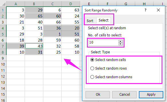
1. Roghnaigh an raon a theastaíonn uait chun uimhreacha randamacha a ghiniúint, agus cliceáil Kutools > Ionsáigh > Cuir isteach Sonraí randamacha. Féach an pictiúr:

2. Sa Cuir isteach Sonraí randamacha dialóg, téigh go dtí an Slánuimhir cluaisín, clóscríobh an raon uimhreacha atá uait sa ó agus Chun boscaí téacs, agus cuimhnigh seiceáil Luachanna uathúla rogha. Féach an pictiúr:

3. cliceáil Ok chun na huimhreacha randamacha a ghiniúint agus an dialóg a fhágáil.

Nóta:Má tá do chealla roghnaithe níos mó ná na huimhreacha randamacha, taispeántar na cealla iomarcacha mar bán.

Is féidir leat an dáta uathúil randamach, am uathúil randamach a chur isteach faoi Cuir isteach Sonraí randamacha. Más mian leat triail saor in aisce de Cuir isteach Sonraí randamacha, le do thoil downloan sé anois!
cuir isteach sonraí randamacha

Leid.Más mian leat sonraí a roghnú nó a shórtáil go randamach, déan iarracht na Kutools a úsáid le haghaidh Excel Raon Sórtáil go randamach mar a thaispeántar sa phictiúr a leanas. Tá sé ag feidhmiú go hiomlán gan teorainn i 30 lá, íoslódáil agus triail saor in aisce anois.

doc a roghnú go randamach


mboilgeog cheart gorm saighead Cuir isteach Sonraí randamacha gan Dúblach


Cuir isteach ticbhoscaí nó cnaipí iolracha go tapa i raon cealla sa bhileog oibre

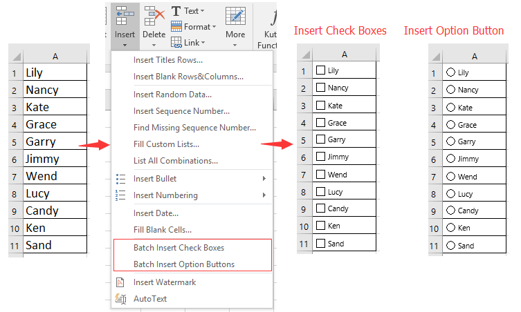
In Excel, ní féidir leat ach bosca seiceála / cnaipe amháin a chur isteach i gcill uair amháin, beidh sé trioblóideach má tá gá le ilchealla a chur isteach i mboscaí seiceála / cnaipí ag an am céanna. Kutools le haghaidh Excel tá fóntais chumhachtach aige - Seiceáil Ionsáigh Baisc Boscaí / Cnaipí Rogha Iontrála Baisc in ann boscaí seiceála / cnaipí a chur isteach sna cealla roghnaithe le cliceáil amháin.  Cliceáil le haghaidh trialach saor in aisce lán-chuimsithe i 30 lá!
cuir isteach cnaipe rogha an bhosca seiceála
 
Kutools for Excel: le níos mó ná 300 breiseán áisiúil Excel, saor in aisce le triail gan aon teorannú i 30 lá.

Uirlisí Táirgiúlachta Oifige is Fearr

🤖 Kutools AI Aide: anailís sonraí a réabhlóidiú bunaithe ar: Forghníomhú Chliste   |  Gin Cód  |  Cruthaigh Foirmlí Saincheaptha  |  Anailís a dhéanamh ar Sonraí agus Cairteacha a Ghin  |  Feidhmeanna Kutools a agairt...
Gnéithe Coitianta: Faigh, Aibhsigh nó Aithnigh Dúblaigh   |  Scrios Sraitheanna Bána   |  Comhcheangail Colúin nó Cealla gan Sonraí a Chailleadh   |   Babhta gan Foirmle ...
Cuardaigh Super: Ilchritéir VLookup    VLookup Illuachanna  |   VLookup Trasna Ilbhileoga   |   Amharc doiléir ....
Liosta anuas Casta: Go tapa Cruthaigh Liosta Anuas   |  Liosta anuas Cleithiúnach   |  Liosta Buail Isteach Ilroghnacha ....
Bainisteoir Colún: Cuir Líon Sonrach Colún leis  |  Colúin Bog  |  Scoránaigh Stádas Infheictheachta na gColún Ceilte  |  Déan comparáid idir Raonta & Colúin ...
Gnéithe Réadmhaoin: Fócas Eangaí   |  Amharc Dearaidh   |   Barra Mór na Foirmle    Leabhar Oibre & Bainisteoir Bileog   |  Leabharlann Acmhainní (Uaththéacs)   |  Piocálaí Dáta   |  Comhcheangail Bileoga Oibre   |  Criptigh/Díchriptigh Cealla    Seol Ríomhphost trí Liosta   |  Scagaire Super   |   Scagaire Speisialta (scagaire trom/iodálach/stailc tríd...) ...
Barr 15 Uirlisí12 Téacs uirlisí (Cuir Téacs, Bain Carachtair,...)   |   50 + Cairt cineálacha (Cairt Gantt,...)   |   40+ Praiticiúil Foirmlí (Ríomh aois bunaithe ar lá breithe,...)   |   19 Insertion uirlisí (Cuir isteach Cód QR, Ionsáigh Pictiúr ón gCosán,...)   |   12 Tiontú uirlisí (Uimhreacha le Focail, Comhshó Airgeadra,...)   |   7 Cumaisc & Scoilt uirlisí (Sraitheanna Comhcheangail Casta, Cealla Scoilt,...)   |   ... agus eile

Supercharge Do Scileanna Excel le Kutools le haghaidh Excel, agus Éifeachtúlacht Taithí Cosúil Ná Roimhe. Kutools le haghaidh Excel Tairiscintí Níos mó ná 300 Ardghnéithe chun Táirgiúlacht a Treisiú agus Sábháil Am.  Cliceáil anseo chun an ghné is mó a theastaíonn uait a fháil ...

Tuairisc


Tugann Tab Oifige comhéadan Tabbed chuig Office, agus Déan Do Obair i bhfad Níos Éasca

  • Cumasaigh eagarthóireacht agus léamh tabbed i Word, Excel, PowerPoint, Foilsitheoir, Rochtain, Visio agus Tionscadal.
  • Oscail agus cruthaigh cáipéisí iolracha i gcluaisíní nua den fhuinneog chéanna, seachas i bhfuinneoga nua.
  • Méadaíonn do tháirgiúlacht 50%, agus laghdaíonn sé na céadta cad a tharlaíonn nuair luch duit gach lá!
Comments (17)
No ratings yet. Be the first to rate!
This comment was minimized by the moderator on the site
En la parte Genere números aleatorios únicos con fórmulas como hago para ampliar el numero de columnas pasar de 2 a 5 sin repetir los numeros segun la formula que ud puso: =IF(ROW()-ROW(A$1)+1>$D$1/2,"",RANK(OFFSET($E$1,ROW()-ROW(A$1)+(COLUMN()-COLUMN($A1))*($D$1/2),),$E$1:INDEX($E$1:$E$1000,$D$1)))
This comment was minimized by the moderator on the site
Hello. I just found this site, and am trying to figure out best way to assign a new code to people. I'd like to assign a random code for people to use between 1000 and 65000, that does not equal any codes already assigned. I'd also like it to be formatted with 5 numbers (00000), but that's not a big deal if it doesn't take care of that. Any ideas on how to make this work? TIA :-)
This comment was minimized by the moderator on the site
Hi, Janel, why you donot try the Data Validation in Excel? It can only allow whole numbers between 1000 and 65000 to be entered in a cell range.
This comment was minimized by the moderator on the site
Help anyone :-) This one I cannot figure out. At our school we often put together students in groups - 2 and 2 together for a number of working sessions. 9 in this case. There are 18 students (vary) in the class. What I am chasing is a formula that gives me a random result of who should work together in the 9 working sessions without having students meeting each other twice. So I need Excel to give me a result of 18 students spread across 9 working sessions and any student must not be match with another student twice. How the xxxx do I fix that? I have search all over the place for inspiration without luck. Any input is appreciated :-)
This comment was minimized by the moderator on the site
Hi, Anders, you need to list all names in column A, then in column B, apply formula =rand(), then specify 2 as the size in cell F2, now apply this formula =ROUNDUP(RANK(B3,$B$3:$B$19)/$F$2,0) in column C as below screenshot shown
This comment was minimized by the moderator on the site
Hi. Thanks for your reply.
I understand you suggestions, but how do I achieve a setup where all students are assigned to maksimum number of workshops where 2 students are randomly assigned to first one workshop, then the second workshop, then the third workshop etc. etc. and to take this even further a student must not be matched with another student that he/she already have worked with. So when having 18 students I need "the system" to allocate all student to (in this case) 9 workshop (e.g. one workshop per week) and no student should be a student they have already worked with.
This comment was minimized by the moderator on the site
Hi there, did you ever manage to work out a solution to this, I've encountered the same issue. Any help would be appreciated.
This comment was minimized by the moderator on the site
Or you could use a sudoku setup.
This comment was minimized by the moderator on the site
How can I do the same thing with a custom list? Not numbers?
This comment was minimized by the moderator on the site
Your custom list is in Column A. Lets say it has 100 values and it is located in A1:A100

Column B is a counter:
1 for B1 and (B1+1) for B2:B100

Column C is a random list:
RAND() for C1:C100

Column D is a random rank based on the random list:
RANK.EQ(C1;$C$1:$C$100)

Column E is your output:
INDEX($A$1:$A$100;MATCH(D1;$B$1:$B$100;0))

Note: There is virtually no chance of generating a duplicate value on column C since RAND() have billions of possibilities. But, if you really want to erase that chance you can type the following formula at column D2:D100
IF(COUNTIFS($C$2:C2;C2)>0;D1+1;RANK.EQ(C2;$C$1:$C$100))
This comment was minimized by the moderator on the site
I need to create 5000 random numbers 1-90 no duplicates 30 columes I and using the formula =RAND() and =IF(ROW()-ROW(A$1)+1>$D$1/2,"",RANK(OFFSET($E$1,ROW()-ROW(A$1)+(COLUMN()-COLUMN($A1))*($D$1/2),),$E$1:INDEX($E$1:$E$1000,$D$1))) is there way that i could change the formula to extract the 5000 numbers
This comment was minimized by the moderator on the site
Sorry I have no idea, you can place this problem to our forum https://www.extendoffice.com/forum.html, maybe someone can help you.
This comment was minimized by the moderator on the site
After about three hours of trying to completely understand the long complicated formula to generate random numbers without duplicates, I figured out a far simpler formula that has the same results. After you randomly generate the numbers in a column using the RAND() function, You can simplify the formula:=IF(ROW()-ROW(A$1)+1>$D$1/2,"",RANK(OFFSET($E$1,ROW()-ROW(A$1)+(COLUMN()-COLUMN($A1))*($D$1/2),),$E$1:INDEX($E$1:$E$1000,$D$1))) in cell a1 to =Rank(E1,$E$1:$E$50). Then if you would like 50 random generated "unique numbers." you simply drag the formula through column a to cell a50. It is a lot simpler. Thank you for answering my question regardless of the huge unneeded formula. If you did not have this website. I don't think I would have been able to solve my problem. #WAR Jiggly
This comment was minimized by the moderator on the site
Actually, if you have two equal values, rank will give the same value to both. Rank formula does return repeated rank values.
This comment was minimized by the moderator on the site
Manuel Ramirez.

The formula RAND() has hundreds of billions of possibilities, but even so you can use a conditional to not repeat the numbers:
A1 = Rank(E1,$E$1:$E$50)
A2 = IF(COUNTIFS($E$1:E1;E1)>1;A1+1;Rank(E2,$E$1:$E$50)
This comment was minimized by the moderator on the site
Hi, Base on Generate unique random numbers with formulas , How can I specify the starting point of a random number? Let's say I want to random "15 to 30".
This comment was minimized by the moderator on the site
Use RANDBETWEEN() to get random numbers lies between two numbers.
There are no comments posted here yet
Please leave your comments in English
Posting as Guest
×
Rate this post:
0   Characters
Suggested Locations