
Conas dátaí formáid choinníollach a dhéanamh níos lú ná / níos mó ná inniu in Excel?

Féadfaidh tú dátaí formáide coinníollach a bhunú bunaithe ar an dáta reatha in Excel. Mar shampla, is féidir leat dátaí a fhormáidiú roimh an lá inniu, nó dátaí níos mó ná an lá inniu a fhormáidiú. Sa rang teagaisc seo, taispeánfaimid duit conas an fheidhm TODAY a úsáid i bhformáidiú coinníollach chun dátaí dlite nó dátaí amach anseo in Excel a aibhsiú go mion.

Dátaí formáid choinníollach roimh an lá inniu nó dátaí amach anseo in Excel


Dátaí formáid choinníollach roimh an lá inniu nó dátaí amach anseo in Excel

Ligean le rá go bhfuil liosta dáta agat mar atá thíos an pictiúr a thaispeántar. Chun na dátaí dlite agus na dátaí amach anseo gan íoc a ligean, déan mar a leanas.

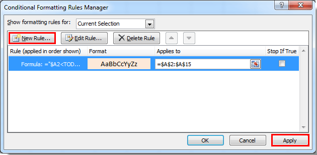
1. Roghnaigh an raon A2: A15, ansin cliceáil Formáidiú Coinníollach > Rialacha a Bhainistiú faoi Baile cluaisín. Féach an pictiúr:

2. Sa Bainisteoir Rialacha Formáidithe Coinníollach bosca dialóige, cliceáil an Riail Nua cnaipe.

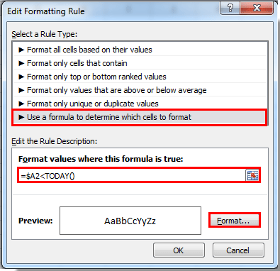
3. Sa Riail Nua Formáidithe bosca dialóige, ní mór duit:

1). Roghnaigh Úsáid foirmle chun a fháil amach cé na cealla atá le formáidiú sa Roghnaigh Cineál Riail alt;

2). Chun formáidiú na dátaí níos sine ná an lá inniu, cóipeáil agus greamaigh an fhoirmle le do thoil = $ A2 isteach sa Luachanna formáide nuair atá an fhoirmle seo fíor bosca;

Do formáidiú na dátaí amach anseo, bain úsáid as an bhfoirmle seo le do thoil = $ A2> TODAY ();

3). Cliceáil ar an déanta cnaipe. Féach an pictiúr:

4. Sa Cealla Formáid bosca dialóige, sonraigh an fhormáid do na dátaí dlite nó dátaí amach anseo, agus ansin cliceáil ar an OK cnaipe.

5. Ansin filleann sé ar an Bainisteoir Rialacha Formáidithe Coinníollach bosca dialóige. Agus cruthaítear riail formáidithe na ndátaí dlite. Más mian leat an riail a chur i bhfeidhm anois, cliceáil ar an Cuir iarratas isteach cnaipe.

6. Ach más mian leat riail na ndátaí dlite agus riail na ndátaí amach anseo a chur i bhfeidhm le chéile, cruthaigh riail nua leis an bhfoirmle formáidithe dáta amach anseo trí na céimeanna thuas a athdhéanamh ó 2 go 4.

7. Nuair a fhillfidh sé ar an Bainisteoir Rialacha Formáidithe Coinníollach bosca dialóige arís, is féidir leat a fheiceáil go bhfuil an dá riail á thaispeáint sa bhosca, cliceáil ar an OK cnaipe chun formáidiú a thosú.

Ansin is féidir leat na dátaí níos sine ná an lá inniu a fheiceáil agus déantar an dáta níos mó ná an lá inniu a fhormáidiú go rathúil.

Formáid choinníollach go héasca gach ró as a chéile sa roghnú:

Kutools le haghaidh Excel's Scáth Malartach Rae / Colún cuidíonn fóntais leat formáidiú coinníollach a chur le gach ró i roghnú Excel.
Íoslódáil rian iomlán saor in aisce 30 lá de Kutools le haghaidh Excel anois!


Earraí gaolmhara:

Uirlisí Táirgiúlachta Oifige is Fearr

🤖 Kutools AI Aide: anailís sonraí a réabhlóidiú bunaithe ar: Forghníomhú Chliste   |  Gin Cód  |  Cruthaigh Foirmlí Saincheaptha  |  Anailís a dhéanamh ar Sonraí agus Cairteacha a Ghin  |  Feidhmeanna Kutools a agairt...
Gnéithe Coitianta: Faigh, Aibhsigh nó Aithnigh Dúblaigh   |  Scrios Sraitheanna Bána   |  Comhcheangail Colúin nó Cealla gan Sonraí a Chailleadh   |   Babhta gan Foirmle ...
Cuardaigh Super: Ilchritéir VLookup    VLookup Illuachanna  |   VLookup Trasna Ilbhileoga   |   Amharc doiléir ....
Liosta anuas Casta: Go tapa Cruthaigh Liosta Anuas   |  Liosta anuas Cleithiúnach   |  Liosta Buail Isteach Ilroghnacha ....
Bainisteoir Colún: Cuir Líon Sonrach Colún leis  |  Colúin Bog  |  Scoránaigh Stádas Infheictheachta na gColún Ceilte  |  Déan comparáid idir Raonta & Colúin ...
Gnéithe Réadmhaoin: Fócas Eangaí   |  Amharc Dearaidh   |   Barra Mór na Foirmle    Leabhar Oibre & Bainisteoir Bileog   |  Leabharlann Acmhainní (Uaththéacs)   |  Piocálaí Dáta   |  Comhcheangail Bileoga Oibre   |  Criptigh/Díchriptigh Cealla    Seol Ríomhphost trí Liosta   |  Scagaire Super   |   Scagaire Speisialta (scagaire trom/iodálach/stailc tríd...) ...
Barr 15 Uirlisí12 Téacs uirlisí (Cuir Téacs, Bain Carachtair,...)   |   50 + Cairt cineálacha (Cairt Gantt,...)   |   40+ Praiticiúil Foirmlí (Ríomh aois bunaithe ar lá breithe,...)   |   19 Insertion uirlisí (Cuir isteach Cód QR, Ionsáigh Pictiúr ón gCosán,...)   |   12 Tiontú uirlisí (Uimhreacha le Focail, Comhshó Airgeadra,...)   |   7 Cumaisc & Scoilt uirlisí (Sraitheanna Comhcheangail Casta, Cealla Scoilt,...)   |   ... agus eile

Supercharge Do Scileanna Excel le Kutools le haghaidh Excel, agus Éifeachtúlacht Taithí Cosúil Ná Roimhe. Kutools le haghaidh Excel Tairiscintí Níos mó ná 300 Ardghnéithe chun Táirgiúlacht a Treisiú agus Sábháil Am.  Cliceáil anseo chun an ghné is mó a theastaíonn uait a fháil ...

Tuairisc


Tugann Tab Oifige comhéadan Tabbed chuig Office, agus Déan Do Obair i bhfad Níos Éasca

  • Cumasaigh eagarthóireacht agus léamh tabbed i Word, Excel, PowerPoint, Foilsitheoir, Rochtain, Visio agus Tionscadal.
  • Oscail agus cruthaigh cáipéisí iolracha i gcluaisíní nua den fhuinneog chéanna, seachas i bhfuinneoga nua.
  • Méadaíonn do tháirgiúlacht 50%, agus laghdaíonn sé na céadta cad a tharlaíonn nuair luch duit gach lá!
Comments (24)
No ratings yet. Be the first to rate!
This comment was minimized by the moderator on the site
I want to highlight a cell if:
1. today's date is greater than the date in another cell or blank (=TODAY()>'APM Tracker'P14) AND ALSO;
2. If the date in P15 is greater than P14 same highlight color AND ALSO;
3. If the date in P15 is less than P14 I do not want the highlight
This comment was minimized by the moderator on the site
Hey All,

I want to get only past due dates in the particular column. Instead of highlighting the cells with color i need the dates to be picked in the column

Any solution for this....
This comment was minimized by the moderator on the site
Alright, I read through this thread and did not see this question asked/answered. I have a column of future dates. I would like to add conditional formatting to flag that date exactly 30 days before (1st color "Hey you should get this done its due in 30 day's") and 7 days ( 2nd color "You procrastinated and now you have 7 days to complete this"). Any help here?
This comment was minimized by the moderator on the site
Hi Michael,
I am not sure I understand your question clearly. If you want to hight the date which is 30 days and 7 days from today. Please use the following formulas to create two formula rules with different highlighted colors:
=D9=TODAY()+30
=D9=TODAY()+7

https://www.extendoffice.com/images/stories/comments/comment-picture-zxm/conditional-formatting.png
If this is not what you need, please attach a screenshot of your data here.
This comment was minimized by the moderator on the site
To ignore cells that have blanks try this:

=AND($A2<>"",$A2<TODAY())

This assumes the cell you have selected is A2 (change this to whatever cell you have currently selected)
To copy this to the applicable cells, change the "Applies to" to the cell range you need.
This comment was minimized by the moderator on the site
Hi Andy Campbell,
Thank you for sharing.
This comment was minimized by the moderator on the site
Hi
I am trying to use condition formatting to allow a cell to be highlighted when an item is past due based on different turn around times (TAT). I have a column with a submitted date which is then used with the #of days from the TAT to automatically give the due date. Using the following formula, =IF(OR(E3="",A3=""),"",DATE(YEAR(A3),MONTH(A3),DAY(A3)+E3))
The condition formatting currently used is "cell value < today()" applies to +$G:$G.
What I would like to do is use the stop if rule to stop the condition formatting if the date entered in column "H" is < or = to todays date.
Thanks Michelle
This comment was minimized by the moderator on the site
if i want highlight the due date with the conditional : today less or equal 30 days from due date
This comment was minimized by the moderator on the site
I am trying to create conditional formatting that will highlight rows older than 14 days in yellow and highlight rows older than 21 days in red. My date column starts in A2, I have the following rules applied, but only yellow is highlighting and just the date column, not the entire row. Can you help? Scott

1. =ISBLANK(A2)=TRUE
2. =A2<TODAY()-14
3. =A2<TODAY()-21
This comment was minimized by the moderator on the site
I want to ignore blank cells which doesn't have a date i.e I do not want blank cells to be highlighted when I am comparing dates<Today(). Please help
This comment was minimized by the moderator on the site
Hi Madhu,
The first method in this artice can help you solve the problem. Please have a try.
https://www.extendoffice.com/documents/excel/2499-excel-conditional-formatting-ignore-blank-zero.html
This comment was minimized by the moderator on the site
1 colum has the dates in it i want another colum to change colour when this formula is applied.

any ideas?
This comment was minimized by the moderator on the site
Hi grant,
Supposing you want to change the cell color in column B based on dates in column A, please select the column B cells (such as B2:B21), and apply the conditional formatting function with the above formulas =$A2>Today() or =$A2<Today().
This comment was minimized by the moderator on the site
Hello! can anyone help me?

I have =TODAY() formula in A1 and need 3 more rules to work as per below

rule 1 all dates 8 to 14 days older than today

rule 2 : all dates older 14 to 30 days than today

rule 3: all dates 31 or more days older than today
This comment was minimized by the moderator on the site
it should be something like this:

if(*cell*+8>Today();if(*cell*+14<Today();"8-14 from today";"N/A"))
There are no comments posted here yet
Load More
Please leave your comments in English
Posting as Guest
×
Rate this post:
0   Characters
Suggested Locations