Conas na 5 luach dheireanacha de cholún a mheánú mar uimhreacha nua ag dul isteach?
In Excel, is féidir leat meán na 5 luach dheireanacha a ríomh go tapa i gcolún leis an bhfeidhm Meán, ach, ó am go ham, ní mór duit uimhreacha nua a iontráil taobh thiar de do bhunsonraí, agus ba mhaith leat go n-athrófaí an meánthoradh go huathoibríoch mar na sonraí nua ag dul isteach. Is é sin le rá, ba mhaith leat go léireodh an meán na 5 uimhir dheireanacha de do liosta sonraí i gcónaí, fiú nuair a chuireann tú uimhreacha leis anois agus arís.
Na 5 luach dheireanacha de cholún ar an meán mar uimhreacha nua ag iontráil le foirmlí
 Na 5 luach dheireanacha de cholún ar an meán mar uimhreacha nua ag iontráil le foirmlí
D’fhéadfadh na foirmlí eagar seo a leanas cabhrú leat an fhadhb seo a réiteach, déan mar a leanas:
Iontráil an fhoirmle seo i gcill bhán:
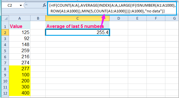
=IF(COUNT(A:A),AVERAGE(INDEX(A:A,LARGE(IF(ISNUMBER(A1:A10000),ROW(A1:A10000)),MIN(5,COUNT(A1:A10000)))):A10000),"no data") (A: A. an colún ina bhfuil na sonraí a d'úsáid tú, A1: A10000 is raon dinimiciúil é, is féidir leat é a leathnú chomh fada le do riachtanas, agus an uimhir 5 léiríonn sé an luach n deireanach.), agus ansin brúigh Ctrl + Shift + Iontráil eochracha le chéile chun meán na 5 uimhir dheireanacha a fháil. Féach an pictiúr:

Agus anois, nuair a ionchuirfidh tú uimhreacha nua taobh thiar de na sonraí bunaidh, athrófar an meán freisin, féach an scáileán:
nótaí: Má tá 0 luach sa cholún cealla, ba mhaith leat na 0 luach a eisiamh ó na 5 uimhir dheireanacha atá agat, ní oibreoidh an fhoirmle thuas, anseo, is féidir liom foirmle eagar eile a thabhairt isteach chun meán na 5 luach neamh-nialasacha deiridh a fháil , iontráil an fhoirmle seo le do thoil:
=AVERAGE(SUBTOTAL(9,OFFSET(A1:A10000,LARGE(IF(A1:A10000>0,ROW(A1:A10000)-MIN(ROW(A1:A10000))),ROW(INDIRECT("1:5"))),0,1))), agus ansin brúigh Ctrl + Shift + Iontráil eochracha chun an toradh a theastaíonn uait a fháil, féach an scáileán:

Earraí gaolmhara:
Conas gach 5 shraith nó cholún in Excel a mheánú?
Conas meánluachanna barr nó bun 3 a fháil in Excel?
Uirlisí Táirgiúlachta Oifige is Fearr
Supercharge Do Scileanna Excel le Kutools le haghaidh Excel, agus Éifeachtúlacht Taithí Cosúil Ná Roimhe. Kutools le haghaidh Excel Tairiscintí Níos mó ná 300 Ardghnéithe chun Táirgiúlacht a Treisiú agus Sábháil Am. Cliceáil anseo chun an ghné is mó a theastaíonn uait a fháil ...
")
Tugann Tab Oifige comhéadan Tabbed chuig Office, agus Déan Do Obair i bhfad Níos Éasca
- Cumasaigh eagarthóireacht agus léamh tabbed i Word, Excel, PowerPoint, Foilsitheoir, Rochtain, Visio agus Tionscadal.
- Oscail agus cruthaigh cáipéisí iolracha i gcluaisíní nua den fhuinneog chéanna, seachas i bhfuinneoga nua.
- Méadaíonn do tháirgiúlacht 50%, agus laghdaíonn sé na céadta cad a tharlaíonn nuair luch duit gach lá!
")