Conas an luach is airde a fháil i gceannteideal colún as a chéile agus ar ais in Excel?
San Airteagal seo, labhróidh mé faoi conas ceanntásc an cholúin den luach is mó i ndiaidh a chéile a chur ar ais in Excel. Mar shampla, tá an raon sonraí seo a leanas agam, is é colún A an bhliain, agus tá na huimhreacha ordaithe ó Eanáir go Bealtaine i gcolún B go F. Agus anois, ba mhaith liom ainm na míosa den luach is mó a fháil i ngach ró.
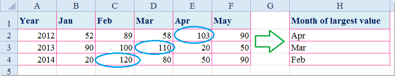
Faigh an luach is airde i ndiaidh a chéile agus ceanntásc an cholúin ar ais leis an bhfoirmle
 Faigh an luach is airde i ndiaidh a chéile agus ceanntásc an cholúin ar ais leis an bhfoirmle
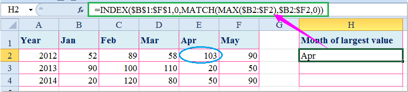
Chun ceanntásc an cholúin den luach is mó i ndiaidh a chéile a aisghabháil, is féidir leat teaglaim d’fheidhmeanna INDEX, MATCH agus MAX a chur i bhfeidhm chun an toradh a fháil. Déan mar a leanas le do thoil:
1. Iontráil an fhoirmle seo i gcill bhán atá uait: =INDEX($B$1:$F$1,0,MATCH(MAX($B2:$F2),$B2:$F2,0)), agus ansin brúigh Iontráil eochair chun ainm na míosa a fháil a mheaitseálann an luach is mó i ndiaidh a chéile. Féach an pictiúr:
2. Ansin roghnaigh an cill agus tarraing an láimhseáil líonta go dtí an raon a theastaíonn uait an fhoirmle seo a bheith ann, féach an pictiúr:

nótaí: San fhoirmle thuas: B1: F1 an bhfuil an tsraith ceanntásca ar mhaith leat filleadh, B2: F2 an raon sonraí ina bhfuil an luach is mó a theastaíonn uait a fháil.
Airteagal gaolmhar:
Conas an luach is airde agus an luach cille cóngarach a fháil in Excel?
Uirlisí Táirgiúlachta Oifige is Fearr
Supercharge Do Scileanna Excel le Kutools le haghaidh Excel, agus Éifeachtúlacht Taithí Cosúil Ná Roimhe. Kutools le haghaidh Excel Tairiscintí Níos mó ná 300 Ardghnéithe chun Táirgiúlacht a Treisiú agus Sábháil Am. Cliceáil anseo chun an ghné is mó a theastaíonn uait a fháil ...
")
Tugann Tab Oifige comhéadan Tabbed chuig Office, agus Déan Do Obair i bhfad Níos Éasca
- Cumasaigh eagarthóireacht agus léamh tabbed i Word, Excel, PowerPoint, Foilsitheoir, Rochtain, Visio agus Tionscadal.
- Oscail agus cruthaigh cáipéisí iolracha i gcluaisíní nua den fhuinneog chéanna, seachas i bhfuinneoga nua.
- Méadaíonn do tháirgiúlacht 50%, agus laghdaíonn sé na céadta cad a tharlaíonn nuair luch duit gach lá!
")