
Conas VLOOKUP a dhéanamh agus luachanna iolracha comhfhreagracha a thabhairt ar ais go cothrománach in Excel?

doc-vlookup-cothrománach-1
De réir réamhshocraithe, is féidir le feidhm VLOOKUP luachanna iolracha comhfhreagracha a thabhairt ar ais ar an leibhéal ingearach in Excel, i gcásanna áirithe, b’fhéidir gur mhaith leat luachanna iolracha a thabhairt ar ais ar leibhéal cothrománach mar atá thíos an pictiúr a thaispeántar. Inseoidh mé duit gur féidir le foirmle an tasc seo a réiteach.
VLOOKUP agus cuir luachanna iolracha ar ais go cothrománach

mboilgeog cheart gorm saighead VLOOKUP agus cuir luachanna iolracha ar ais go cothrománach

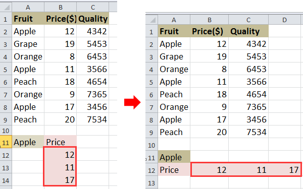
Mar shampla, tá raon sonraí agat mar atá thíos an pictiúr a thaispeántar, agus ba mhaith leat praghsanna Apple a VLOOKUP.
doc-vlookup-cothrománach-2

1. Roghnaigh cill agus clóscríobh an fhoirmle seo =INDEX($B$2:$B$9, SMALL(IF($A$11=$A$2:$A$9, ROW($A$2:$A$9)-ROW($A$2)+1), COLUMN(A1))) isteach dó, agus ansin brúigh Shift + Ctrl + Iontráil agus tarraing an láimhseáil autofill ar dheis chun an fhoirmle seo a chur i bhfeidhm go dtí #NUM! le feiceáil. Féach an pictiúr:
doc-vlookup-cothrománach-3

2. Ansin scrios an #NUM !. Féach an pictiúr:
doc-vlookup-cothrománach-4

Leid: San fhoirmle thuas, is é B2: B9 an raon colún ar mhaith leat na luachanna a thabhairt ar ais ann, is é A2: A9 an raon colún a bhfuil an luach cuardaigh ann, is é A11 an luach amharc, is é A1 an chéad chill de do raon sonraí , Is é A2 an chéad chill den raon colún a bhfuil an luach amharc agat air.

Más mian leat luachanna iolracha a thabhairt ar ais go hingearach, is féidir leat an t-alt seo a léamh Conas luach a chuardach ar aisluachanna comhfhreagracha iolracha in Excel?


Comhcheangail go héasca bileoga iolracha / Leabhar Oibre in aon bhileog amháin nó Leabhar Oibre

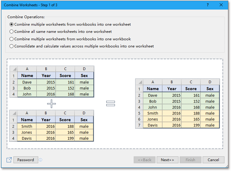
D’fhéadfadh go mbeadh bileoga nó leabhair oibre le chéile in aon bhileog amháin nó leabhar oibre in Excel, ach leis an Chomhcheangail feidhm i Kutools le haghaidh Excel, is féidir leat an iliomad bileoga / leabhar oibre a chumasc i mbileog amháin nó i leabhar oibre, freisin, is féidir leat na bileoga a chomhdhlúthú i gceann amháin le cúpla cad a tharlaíonn.  Cliceáil le haghaidh trialach saor in aisce 30 lá le feiceáil go hiomlán!
bileoga a chur le chéile
 
Kutools for Excel: le níos mó ná 300 breiseán áisiúil Excel, saor in aisce le triail gan aon teorannú i 30 lá.

Uirlisí Táirgiúlachta Oifige is Fearr

🤖 Kutools AI Aide: anailís sonraí a réabhlóidiú bunaithe ar: Forghníomhú Chliste   |  Gin Cód  |  Cruthaigh Foirmlí Saincheaptha  |  Anailís a dhéanamh ar Sonraí agus Cairteacha a Ghin  |  Feidhmeanna Kutools a agairt...
Gnéithe Coitianta: Faigh, Aibhsigh nó Aithnigh Dúblaigh   |  Scrios Sraitheanna Bána   |  Comhcheangail Colúin nó Cealla gan Sonraí a Chailleadh   |   Babhta gan Foirmle ...
Cuardaigh Super: Ilchritéir VLookup    VLookup Illuachanna  |   VLookup Trasna Ilbhileoga   |   Amharc doiléir ....
Liosta anuas Casta: Go tapa Cruthaigh Liosta Anuas   |  Liosta anuas Cleithiúnach   |  Liosta Buail Isteach Ilroghnacha ....
Bainisteoir Colún: Cuir Líon Sonrach Colún leis  |  Colúin Bog  |  Scoránaigh Stádas Infheictheachta na gColún Ceilte  |  Déan comparáid idir Raonta & Colúin ...
Gnéithe Réadmhaoin: Fócas Eangaí   |  Amharc Dearaidh   |   Barra Mór na Foirmle    Leabhar Oibre & Bainisteoir Bileog   |  Leabharlann Acmhainní (Uaththéacs)   |  Piocálaí Dáta   |  Comhcheangail Bileoga Oibre   |  Criptigh/Díchriptigh Cealla    Seol Ríomhphost trí Liosta   |  Scagaire Super   |   Scagaire Speisialta (scagaire trom/iodálach/stailc tríd...) ...
Barr 15 Uirlisí12 Téacs uirlisí (Cuir Téacs, Bain Carachtair,...)   |   50 + Cairt cineálacha (Cairt Gantt,...)   |   40+ Praiticiúil Foirmlí (Ríomh aois bunaithe ar lá breithe,...)   |   19 Insertion uirlisí (Cuir isteach Cód QR, Ionsáigh Pictiúr ón gCosán,...)   |   12 Tiontú uirlisí (Uimhreacha le Focail, Comhshó Airgeadra,...)   |   7 Cumaisc & Scoilt uirlisí (Sraitheanna Comhcheangail Casta, Cealla Scoilt,...)   |   ... agus eile

Supercharge Do Scileanna Excel le Kutools le haghaidh Excel, agus Éifeachtúlacht Taithí Cosúil Ná Roimhe. Kutools le haghaidh Excel Tairiscintí Níos mó ná 300 Ardghnéithe chun Táirgiúlacht a Treisiú agus Sábháil Am.  Cliceáil anseo chun an ghné is mó a theastaíonn uait a fháil ...

Tuairisc


Tugann Tab Oifige comhéadan Tabbed chuig Office, agus Déan Do Obair i bhfad Níos Éasca

  • Cumasaigh eagarthóireacht agus léamh tabbed i Word, Excel, PowerPoint, Foilsitheoir, Rochtain, Visio agus Tionscadal.
  • Oscail agus cruthaigh cáipéisí iolracha i gcluaisíní nua den fhuinneog chéanna, seachas i bhfuinneoga nua.
  • Méadaíonn do tháirgiúlacht 50%, agus laghdaíonn sé na céadta cad a tharlaíonn nuair luch duit gach lá!
Comments (20)
No ratings yet. Be the first to rate!
This comment was minimized by the moderator on the site
This article says this uses VLOOKUP, but it uses INDEX... which does not help me. I need a solution for multiple values using VLOOKUP or XLOOKUP in tables.
This comment was minimized by the moderator on the site
you can use TEXTSPLIT function followed by TEXTJOIN FUNCTION in excel 365
This comment was minimized by the moderator on the site
For anyone experiencing issues in a big data range, ensure you dont have any cells existent with "#N/A" or it will break it. Simple error but can be overlooked.
This comment was minimized by the moderator on the site
Hello, I want to use keyword instead of specific text or value here for multiple return values, can you please share code formula for same.
This comment was minimized by the moderator on the site
Hello - This formula worked perfectly - thank you! However, I want to apply it to a long list of lookup values. When I copy and paste the formula it obviously returns the same results as the first lookup value so I removed the $'s from $A$11, but that changes the result to something incorrect. How can I quickly apply this same formula for a long list of lookup values?

Thank you!

M
This comment was minimized by the moderator on the site
Bonjour,

J'ai retransposé mon problème exactement dans les mêmes positions de colonne que l'exemple et j’obtiens le message #VALEUR! dès la première case.

Mon excel fonctionne en francais, j'ai tout retranscrit en francais, passé ";"au lieu de ",", appuyé sur CTRL+MAJ+Entrée... des idées sur l'origine du problème?

Fanny
This comment was minimized by the moderator on the site
what you want to put the price in order of highest qty from column c?
This comment was minimized by the moderator on the site
i have to find vertical value first, in vertical value there are more horizontal value and i have choose grater value which i have. which function or formula can help
This comment was minimized by the moderator on the site
Hi. I have three google spreadsheet. First sheet is named "Summary. It is a table containing the name of our employee and number of evaluation in a week from 1-7. The next sheet is named "Chat Score"and third sheet is named Ëmail Score". What I want to to do is when we input a evaluation score to one of our employee it will be automatically recorded on the "Summary sheet" as evaluation 1 or 2 and so on and so forth. In short I want to get multiple return value in a single seach key across multiple sheet. I hope you can help. https://docs.google.com/spreadsheets/d/1lt-e4MxddUKg5xDt_0YchBiEgGe4mFKB-dHENwwtA6Y/edit?usp=sharing

https://docs.google.com/spreadsheets/d/1lt-e4MxddUKg5xDt_0YchBiEgGe4mFKB-dHENwwtA6Y/edit?usp=sharing
This comment was minimized by the moderator on the site
Although I'm looking up my values in another worksheet (I don't think this should cause a problem?), I only seem to have success dragging to the right if I go in and change the +1 to '0' for the 1st instance of the lookup ID, '1' for the 2nd instance and so on. I know how many instances of the lookup ID I have so I can workaround. What do I need to change to allow me to successfully drag the fx across horizontally without needing to edit (i.e getting the #NUM to appear once there are no more lookup values to return).
This comment was minimized by the moderator on the site
Sorry, I have not found any solutions about your problems. If you have found that, could you tell me? Thank u.
This comment was minimized by the moderator on the site
Change Column to Row at the end of the formula

"=INDEX($B$1:$B$206, SMALL(IF($A$209=$A$1:$A$206, ROW($A$1:$A$206)-ROW($A$1)+1), ROW(A1)))"
This comment was minimized by the moderator on the site
How to List all values(like list of groceries bought) caused by a specific value (by a person X) using VLOOK_UP and other possible formulas
This comment was minimized by the moderator on the site
You mean that to list all grocerise a person need to buy, right? If so, you can refer to the formula in this article, and change the arguments as you need as below screenshot shown.
There are no comments posted here yet
Load More
Please leave your comments in English
Posting as Guest
×
Rate this post:
0   Characters
Suggested Locations