
Conas an dáta a shlánú go dtí an lá seachtaine roimhe sin nó an chéad lá seachtaine eile in Excel?

doc-rabh-go-roimhe-dé Domhnaigh-1
Uaireanta, b’fhéidir go mbeidh ort an lá seachtaine sonrach roimhe sin nó an chéad lá eile ar nós an Domhnaigh a fháil bunaithe ar dháta mar a léirítear an seat scáileáin ar chlé. Anseo soláthraíonn an teagasc seo dhá fhoirmle chun an post seo a láimhseáil go héasca in Excel.
Dáta slánaithe go dtí an chéad lá seachtaine sonrach eile
Dáta slánaithe go dtí an lá sonrach seachtaine roimhe sin

mboilgeog cheart gorm saighead Dáta slánaithe go dtí an chéad Lá seachtaine sonrach eile

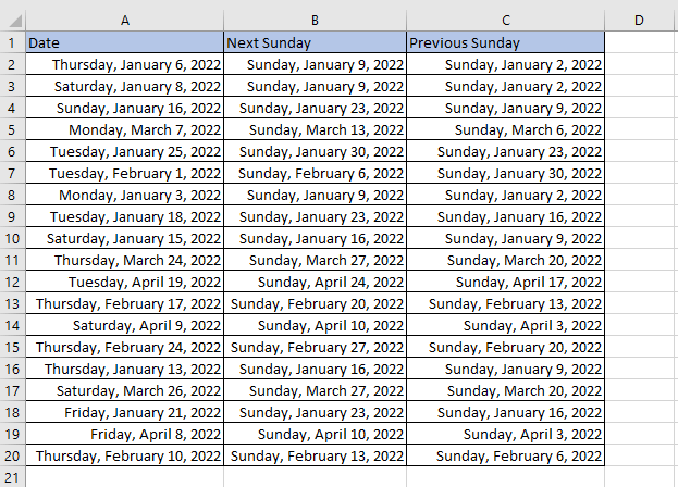
Mar shampla, anseo chun an chéad Domhnach eile a fháil de na dátaí i gcolún A

1. Roghnaigh cill ar mhaith leat a chur ar an gcéad dáta Dé Domhnaigh seo chugainn, ansin greamaigh nó cuir isteach thíos an fhoirmle:

=IF(MOD(A2-1,7)>7,A2+7-MOD(A2-1,7)+7,A2+7-MOD(A2-1,7))

2. Ansin brúigh Iontráil eochair chun an chéad Domhnach seo chugainn a fháil, a thaispeánfar mar uimhir 5 dhigit, ansin tarraing líonadh uathoibríoch síos chun na torthaí go léir a fháil.

doc-rabh-go-roimhe-dé Domhnaigh-1

3. Ansin coinnigh na cealla foirmle roghnaithe, brúigh Ctrl + 1 eochracha chun an Cealla Formáid dialóg, ansin faoi Uimhir tab, roghnaigh dáta agus roghnaigh cineál dáta amháin ón liosta ceart mar is gá duit. Cliceáil OK.

doc-rabh-go-roimhe-dé Domhnaigh-1

Anois tá torthaí na foirmle léirithe i bhformáid dáta.

doc-rabh-go-roimhe-dé Domhnaigh-1

Chun an chéad lá eile den tseachtain a fháil, bain úsáid as na foirmlí thíos:

Lá seachtaine Foirmle
Dé Domhnaigh =IF(MOD(A2-1,7)>7,A2+7-MOD(A2-1,7)+7,A2+7-MOD(A2-1,7))
Dé Sathairn =IF(MOD(A2-1,7)>6,A2+6-MOD(A2-1,7)+7,A2+6-MOD(A2-1,7))
Dé hAoine =IF(MOD(A2-1,7)>5,A2+5-MOD(A2-1,7)+7,A2+5-MOD(A2-1,7))
Déardaoin =IF(MOD(A2-1,7)>4,A2+4-MOD(A2-1,7)+7,A2+4-MOD(A2-1,7))
Dé Céadaoin =IF(MOD(A1-1,7)>3,A1+3-MOD(A1-1,7)+7,A1+3-MOD(A1-1,7))
;Dé Máirt =IF(MOD(A1-1,7)>2,A1+2-MOD(A1-1,7)+7,A1+2-MOD(A1-1,7))
Dé Luain =IF(MOD(A1-1,7)>1,A1+1-MOD(A1-1,7)+7,A1+1-MOD(A1-1,7))

mboilgeog cheart gorm saighead Dáta slánaithe go dtí an lá sonrach seachtaine roimhe sin

Mar shampla, anseo chun an Domhnach roimhe sin de na dátaí i gcolún A a fháil

1. Roghnaigh cill ar mhaith leat a chur ar an gcéad dáta Dé Domhnaigh seo chugainn, ansin greamaigh nó cuir isteach thíos an fhoirmle:

=A2- LÁ SEACHTAIN(A2,2)

2. Ansin brúigh Iontráil eochair chun an chéad Domhnach seo chugainn a fháil, ansin tarraing líonadh uathoibríoch síos chun na torthaí go léir a fháil.

doc-rabh-go-roimhe-dé Domhnaigh-1

Más mian leat an fhormáid dáta a athrú, coinnigh na cealla foirmle roghnaithe, brúigh Ctrl + 1 eochracha chun an Cealla Formáid dialóg, ansin faoi Uimhir tab, roghnaigh dáta agus roghnaigh cineál dáta amháin ón liosta ceart mar is gá duit. Cliceáil OK.

doc-rabh-go-roimhe-dé Domhnaigh-1

Anois tá torthaí na foirmle léirithe i bhformáid dáta.

doc-rabh-go-roimhe-dé Domhnaigh-1

Chun lá seachtaine eile a fháil roimhe seo, bain úsáid as na foirmlí thíos:

Lá seachtaine Foirmle
Dé Domhnaigh =A2- LÁ SEACHTAIN(A2,2)
Dé Sathairn =IF(WEEKDAY(A2,2)>6,A2-WEEKDAY(A2,1),A2-WEEKDAY(A2,2)-1)
Dé hAoine =IF(WEEKDAY(A2,2)>5,A2-WEEKDAY(A2,2)+5,A2-WEEKDAY(A2,2)-2)
Déardaoin =IF(WEEKDAY(A2,2)>4,A2-WEEKDAY(A2,2)+4,A2-WEEKDAY(A2,2)-3)
Dé Céadaoin =IF(WEEKDAY(A2,2)>3,A2-WEEKDAY(A2,2)+3,A2-WEEKDAY(A2,2)-4)
;Dé Máirt =IF(WEEKDAY(A2,2)>2,A2-WEEKDAY(A2,2)+2,A2-WEEKDAY(A2,2)-5)
Dé Luain =IF(WEEKDAY(A2,2)>1,A2-WEEKDAY(A2,2)+1,A2-WEEKDAY(A2,2)-6)

Cúntóir Cumhachtach Dáta & Am

An Dáta & Am Cúntóir gné de Kutools le haghaidh Excel, tacaíonn sé go héasca am dáta a shuimiú/a dhealú, an difríocht idir dhá dháta a ríomh, agus aois a ríomh bunaithe ar lá breithe.  Cliceáil le haghaidh trialach saor in aisce!
doc-rabh-go-roimhe-dé Domhnaigh-1
 
Kutools le haghaidh Excel: le níos mó ná 200 breiseán handy Excel, saor in aisce chun iarracht a dhéanamh gan aon teorainn.

Uirlisí Táirgiúlachta Oifige is Fearr

🤖 Kutools AI Aide: anailís sonraí a réabhlóidiú bunaithe ar: Forghníomhú Chliste   |  Gin Cód  |  Cruthaigh Foirmlí Saincheaptha  |  Anailís a dhéanamh ar Sonraí agus Cairteacha a Ghin  |  Feidhmeanna Kutools a agairt...
Gnéithe Coitianta: Faigh, Aibhsigh nó Aithnigh Dúblaigh   |  Scrios Sraitheanna Bána   |  Comhcheangail Colúin nó Cealla gan Sonraí a Chailleadh   |   Babhta gan Foirmle ...
Cuardaigh Super: Ilchritéir VLookup    VLookup Illuachanna  |   VLookup Trasna Ilbhileoga   |   Amharc doiléir ....
Liosta anuas Casta: Go tapa Cruthaigh Liosta Anuas   |  Liosta anuas Cleithiúnach   |  Liosta Buail Isteach Ilroghnacha ....
Bainisteoir Colún: Cuir Líon Sonrach Colún leis  |  Colúin Bog  |  Scoránaigh Stádas Infheictheachta na gColún Ceilte  |  Déan comparáid idir Raonta & Colúin ...
Gnéithe Réadmhaoin: Fócas Eangaí   |  Amharc Dearaidh   |   Barra Mór na Foirmle    Leabhar Oibre & Bainisteoir Bileog   |  Leabharlann Acmhainní (Uaththéacs)   |  Piocálaí Dáta   |  Comhcheangail Bileoga Oibre   |  Criptigh/Díchriptigh Cealla    Seol Ríomhphost trí Liosta   |  Scagaire Super   |   Scagaire Speisialta (scagaire trom/iodálach/stailc tríd...) ...
Barr 15 Uirlisí12 Téacs uirlisí (Cuir Téacs, Bain Carachtair,...)   |   50 + Cairt cineálacha (Cairt Gantt,...)   |   40+ Praiticiúil Foirmlí (Ríomh aois bunaithe ar lá breithe,...)   |   19 Insertion uirlisí (Cuir isteach Cód QR, Ionsáigh Pictiúr ón gCosán,...)   |   12 Tiontú uirlisí (Uimhreacha le Focail, Comhshó Airgeadra,...)   |   7 Cumaisc & Scoilt uirlisí (Sraitheanna Comhcheangail Casta, Cealla Scoilt,...)   |   ... agus eile

Supercharge Do Scileanna Excel le Kutools le haghaidh Excel, agus Éifeachtúlacht Taithí Cosúil Ná Roimhe. Kutools le haghaidh Excel Tairiscintí Níos mó ná 300 Ardghnéithe chun Táirgiúlacht a Treisiú agus Sábháil Am.  Cliceáil anseo chun an ghné is mó a theastaíonn uait a fháil ...

Tuairisc


Tugann Tab Oifige comhéadan Tabbed chuig Office, agus Déan Do Obair i bhfad Níos Éasca

  • Cumasaigh eagarthóireacht agus léamh tabbed i Word, Excel, PowerPoint, Foilsitheoir, Rochtain, Visio agus Tionscadal.
  • Oscail agus cruthaigh cáipéisí iolracha i gcluaisíní nua den fhuinneog chéanna, seachas i bhfuinneoga nua.
  • Méadaíonn do tháirgiúlacht 50%, agus laghdaíonn sé na céadta cad a tharlaíonn nuair luch duit gach lá!
Comments (16)
No ratings yet. Be the first to rate!
This comment was minimized by the moderator on the site
I have tested this but partially incorrect result was out. Why ?
I wanted to get next Friday.

=IF(A2="","",A2+5-Mod(A2-1,7))

I have entered 11/19/2022
The result was past day 11/18/2022
This comment was minimized by the moderator on the site
Thanks for your reminder, the original formula is not enough rigorous indeed. I have updated the formulas and rewrited the tutorial, hope the new formulas can help you.
This comment was minimized by the moderator on the site
Im trying to work out how to use a date, less an amount of days but ensure when subtracting the days it lands on a weekday not a weekend.
Any formulas??
This comment was minimized by the moderator on the site
Hi Everyone,
I use the formula below to round to the next Thursday where A1 is the cell with your original date and 14 is for Thursday. You can use other numbers for other days if required. 11=Monday, 12=Tuesday, 13=Wednesday, etc...

Also, you can use a 1 instead of an 8 to get the Thursday before your original date in A1. If your original date is already a Thursday the formula will produce the same date as in A1.

I hope this helps!

=A1+(0-WEEKDAY(A1,14)+8)
This comment was minimized by the moderator on the site
Thank you! This worked :)
This comment was minimized by the moderator on the site
I put this into google sheets and to make the dates become next thursday but I have not been able to get it to work especially for the dates right after thursdays. =IF(L2="","",L2+4-MOD(L2-1,4)) is the function i used to make it thursday but not all dates were thursday.
This comment was minimized by the moderator on the site
to clarify, all dates become thursday, but friday and saturday will not convert to the next weeks thursday instead they will go back a day or two to the previous thursday instead going to next weeks thursday, is there any way to fix this in the function =IF(L4="","",L4+4-MOD(L4-1,7))
This comment was minimized by the moderator on the site
Hi Kisho,

I use the formula below to round to the next Thursday where A1 is the cell with your original date and 14 is for Thursday. You can use other numbers for other days if required. 11=Monday, 12=Tuesday, 13=Wednesday, etc...

Also, you can use a 1 instead of an 8 to get the Thursday before your original date in A1. If your original date is already a Thursday the formula will produce the same date as in A1.

I hope this helps!

=A1+(0-WEEKDAY(A1,14)+8)
This comment was minimized by the moderator on the site
Hi Kisho,
I use the formula below to round to the next Thursday where A1 is the cell with your original date and 14 is for Thursday. You can use other numbers for other days if required. 11=Monday, 12=Tuesday, 13=Wednesday, etc...
Also, you can use a 1 instead of an 8 to get the Thursday before your original date in A1. If your original date is already a Thursday the formula will produce the same date as in A1.
I hope this helps!
=A1+(0-WEEKDAY(A1,14)+8)
This comment was minimized by the moderator on the site
I put this into google sheets and to make the dates become next thursday but I have not been able to get it to work especially for the dates right after thursdays. =IF(L2="","",L2+4-MOD(L2-1,4)) is the function i used to make it thursday but not all dates were thursday.
This comment was minimized by the moderator on the site
Si quiero la fecha del próximo viernes cómo debo modificar las variables? Gracias
This comment was minimized by the moderator on the site
Sorry, I cannot understand, could you speak in English?
This comment was minimized by the moderator on the site
hi guys,

I used the formula below, I hope it works for you.
IF(WEEKDAY(H2,16)<>7,(7-WEEKDAY(H2,16))+H2,H2) where H2 is the date that you want to round up to the next day of the week (in my case for Friday) and the 16 is the format to start the date with Saturday as #1 and Friday as #7.
This comment was minimized by the moderator on the site
Your round to previous Sunday is flawed. Even shows as much on your sheet.
This comment was minimized by the moderator on the site
So, what would be the correct formula to first check to see if a cell has a date, else leave it blank and make the date the fall on a Friday before if the date falls on a Saturday or Sunday?
This comment was minimized by the moderator on the site
I found a workaround for to the previous Friday. You can change the switch "results" as needed to round to different days.=H3-SWITCH(TEXT(H3, "DDD"), "Mon", 3, "Tue", 4, "Wed", 5, "Thu", 6, "Fri", 0, "Sat", 1, "Sun", 2)
=[date]-SWITCH(TEXT([date], "DDD"), "Mon", 3, "Tue", 4, "Wed", 5, "Thu", 6, "Fri", 0, "Sat", 1, "Sun", 2)
There are no comments posted here yet
Please leave your comments in English
Posting as Guest
×
Rate this post:
0   Characters
Suggested Locations