Conas cealla a chónascadh má tá an luach céanna ann i gcolún eile in Excel?
Mar a thaispeántar sa screenshot thíos, más mian leat cealla a chomhcheangal sa dara colún bunaithe ar na luachanna céanna sa chéad cholún, tá roinnt modhanna ann ar féidir leat a úsáid. San Airteagal seo, tabharfaimid isteach trí bhealach chun an tasc seo a chur i gcrích.

Cealla concatenate má tá an luach céanna le foirmlí agus scagaire
Cuidíonn na foirmlí seo a leanas le hábhar na gcealla comhfhreagracha a chomhcheangal i gcolún bunaithe ar an luach céanna i gcolún eile.
1. Roghnaigh cill bhán seachas an dara colún (anseo roghnaímid cill C2), iontráil an fhoirmle = IF (A2 <> A1, B2, C1 & "," & B2) isteach sa bharra foirmle, agus ansin brúigh an Iontráil eochair.

2. Ansin roghnaigh cill C2, agus tarraing an Láimhseáil Líon isteach go dtí na cealla a theastaíonn uait a chomhchuibhiú.

3. Iontráil foirmle = IF (A2 <> A3, CONCATENATE (A2, "," "", C2, "" ""), "") isteach i gcill D2, agus tarraing Líon Líon Láimhseáil síos go dtí na cealla scíthe.

4. Roghnaigh cill D1, agus cliceáil Dáta > scagairí. Féach an pictiúr:

5. Cliceáil ar an saighead anuas i gcill D1, dícheangail an (Falamh) bosca, agus ansin cliceáil ar an OK cnaipe.

Feiceann tú go bhfuil na cealla comhtháthaithe má tá luachanna an chéad cholúin mar an gcéanna.

nótaí: Chun na foirmlí thuas a úsáid go rathúil, caithfidh na luachanna céanna i gcolún A a bheith leanúnach.
Cealla a chomhchuibhiú go héasca má tá an luach céanna acu le Kutools for Excel (roinnt cad a tharlaíonn)
Éilíonn an modh a thuairiscítear thuas dhá cholún cúntóir a chruthú agus tá céimeanna iolracha i gceist, rud a d'fhéadfadh a bheith deacair. Má tá bealach níos simplí á lorg agat, smaoinigh ar úsáid a bhaint as an Sraitheanna Comhcheangail Casta uirlis ó Kutools le haghaidh Excel. Gan ach cúpla cad a tharlaíonn, ceadaíonn an áirgiúlacht seo duit cealla a chomhcheangail trí úsáid a bhaint as teorannóir ar leith, rud a fhágann go bhfuil an próiseas tapa agus gan stró.
Leid: Sula gcuirfidh tú an uirlis seo i bhfeidhm, suiteáil le do thoil Kutools le haghaidh Excel ar dtús. Téigh go dtína íoslódáil saor in aisce anois.
- Roghnaigh an raon is mian leat a chomhcheangail;
- Socraigh an colún leis na luachanna céanna leis an Eochair Bhunscoile colún.
- Sonraigh deighilteoir chun na cealla a chomhcheangal.
- cliceáil OK.
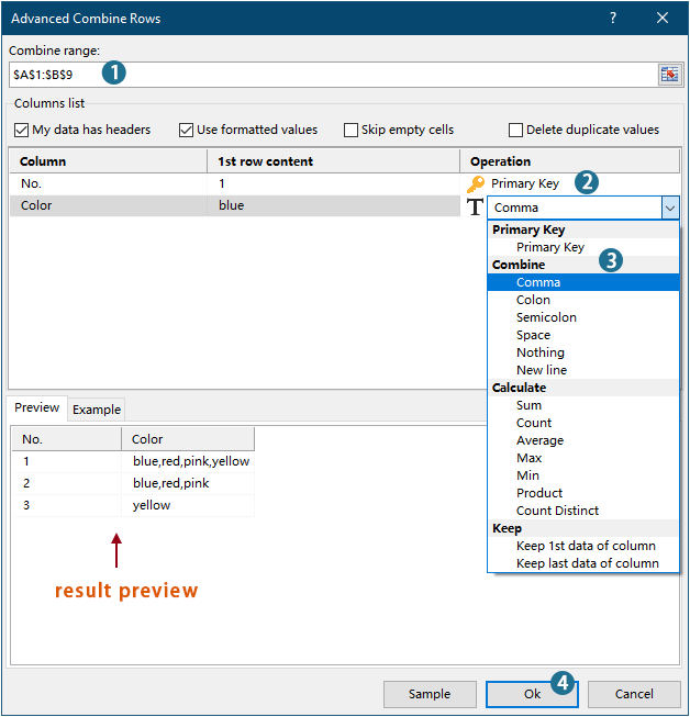
Toradh

- Chun an ghné seo a chur i bhfeidhm, le do thoil Íoslódáil agus a shuiteáil Kutools do Excel an chéad.
- Chun tuilleadh eolais a fháil faoin ngné seo, féach ar an alt seo: Comhcheangail na luachanna céanna go tapa nó déan sraitheanna dúblacha in Excel
Cealla concatenate má tá an luach céanna le cód VBA
Is féidir leat cód VBA a úsáid freisin chun cealla a chomhcheangal i gcolún má tá an luach céanna i gcolún eile.
1. Brúigh Eile + F11 eochracha a oscailt Feidhmchláir Bhunúsacha Amharc Microsoft fhuinneog.
2. Sa Feidhmchláir Bhunúsacha Amharc Microsoft fuinneog, cliceáil Ionsáigh > Modúil. Ansin cóipeáil agus greamaigh thíos an cód isteach sa Modúil fhuinneog.
Cód VBA: cealla comhthráthacha má tá na luachanna céanna acu
Sub ConcatenateCellsIfSameValues()
	Dim xCol As New Collection
	Dim xSrc As Variant
	Dim xRes() As Variant
	Dim I As Long
	Dim J As Long
	Dim xRg As Range
	xSrc    = Range("A1", Cells(Rows.Count, "A").End(xlUp)).Resize(, 2)
	Set xRg = Range("D1")
	On Error Resume Next
	For I = 2 To UBound(xSrc)
		xCol.Add xSrc(I, 1), TypeName(xSrc(I, 1)) & CStr(xSrc(I, 1))
	Next I
	On Error GoTo 0
	ReDim xRes(1 To xCol.Count + 1, 1 To 2)
	xRes(1, 1) = "No"
	xRes(1, 2) = "Combined Color"
	For I = 1 To xCol.Count
		xRes(I + 1, 1) = xCol(I)
		For J = 2 To UBound(xSrc)
			If xSrc(J, 1) = xRes(I + 1, 1) Then
				xRes(I + 1, 2) = xRes(I + 1, 2) & ", " & xSrc(J, 2)
			End If
		Next J
		xRes(I + 1, 2) = Mid(xRes(I + 1, 2), 2)
	Next I
	Set xRg = xRg.Resize(UBound(xRes, 1), UBound(xRes, 2))
	xRg.NumberFormat = "@"
	xRg = xRes
	xRg.EntireColumn.AutoFit
End Subnótaí:
3. Brúigh an F5 eochair chun an cód a rith, ansin gheobhaidh tú na torthaí comhtháthaithe i raon sonraithe.

Cealla concatenate go héasca má tá an luach céanna le Kutools le haghaidh Excel
Uirlisí Táirgiúlachta Oifige is Fearr
Supercharge Do Scileanna Excel le Kutools le haghaidh Excel, agus Éifeachtúlacht Taithí Cosúil Ná Roimhe. Kutools le haghaidh Excel Tairiscintí Níos mó ná 300 Ardghnéithe chun Táirgiúlacht a Treisiú agus Sábháil Am. Cliceáil anseo chun an ghné is mó a theastaíonn uait a fháil ...
")
Tugann Tab Oifige comhéadan Tabbed chuig Office, agus Déan Do Obair i bhfad Níos Éasca
- Cumasaigh eagarthóireacht agus léamh tabbed i Word, Excel, PowerPoint, Foilsitheoir, Rochtain, Visio agus Tionscadal.
- Oscail agus cruthaigh cáipéisí iolracha i gcluaisíní nua den fhuinneog chéanna, seachas i bhfuinneoga nua.
- Méadaíonn do tháirgiúlacht 50%, agus laghdaíonn sé na céadta cad a tharlaíonn nuair luch duit gach lá!
")