
Conas luachanna uathúla a bhaint amach bunaithe ar chritéir in Excel?

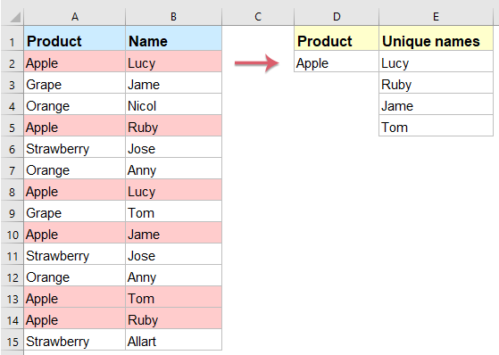
Ag ceapadh, tá an raon sonraí clé agat nach dteastaíonn uait ach ainmneacha uathúla cholún B a liostáil bunaithe ar chritéar sonrach de cholún A chun an toradh a fháil mar a thaispeántar thíos. Conas a d’fhéadfá déileáil leis an tasc seo in Excel go tapa agus go héasca?

Sliocht luachanna uathúla bunaithe ar chritéir le foirmle eagar

Sliocht luachanna uathúla bunaithe ar chritéir iolracha le foirmle eagar

Bain luachanna uathúla ó liosta cealla a bhfuil gné úsáideach acu


Sliocht luachanna uathúla bunaithe ar chritéir le foirmle eagar

Chun an post seo a réiteach, is féidir leat foirmle eagar casta a chur i bhfeidhm, déan mar a leanas:

1. Cuir isteach an fhoirmle thíos i gcill bhán inar mian leat an toradh eastósctha a liostáil, sa sampla seo, cuirfidh mé é go cill E2, agus ansin brúigh Shift + Ctrl + Iontráil eochracha chun an chéad luach uathúil a fháil.

=IFERROR(INDEX($B$2:$B$15, MATCH(0, IF($D$2=$A$2:$A$15, COUNTIF($E$1:$E1, $B$2:$B$15), ""), 0)),"")

2. Ansin, tarraing an láimhseáil líonta síos go dtí na cealla go dtí go dtaispeántar cealla bána, agus anois go bhfuil na luachanna uathúla uile bunaithe ar an gcritéar sonrach liostaithe, féach an scáileán:

Nóta: San fhoirmle thuas: B2: B15 an bhfuil na luachanna uathúla ar mhaith leat a bhaint astu sa raon colún, A2: A15 an bhfuil an critéar ar a bhfuil tú bunaithe sa cholún, D2 léiríonn sé an critéar ar mhaith leat na luachanna uathúla a liostáil bunaithe ar, agus E1 an bhfuil an chill os cionn na foirmle a iontráladh agat.

Sliocht luachanna uathúla bunaithe ar chritéir iolracha le foirmle eagar

Más mian leat na luachanna uathúla a bhaint amach bunaithe ar dhá choinníoll, seo foirmle eagair eile ar féidir leat fabhar a dhéanamh duit, déan mar seo le do thoil:

1. Iontráil an fhoirmle thíos i gcill bhán inar mian leat na luachanna uathúla a liostáil, sa sampla seo, cuirfidh mé é go cill G2, agus ansin brúigh Shift + Ctrl + Iontráil eochracha chun an chéad luach uathúil a fháil.

=IFERROR(INDEX($C$2:$C$15,MATCH(0,COUNTIF(G1:$G$1,$C$2:$C$15)+IF($A$2:$A$15<>$E$2,1,0)+IF($B$2:$B$15<>$F$2,1,0),0)),"")

2. Ansin, tarraing an láimhseáil líonta síos go dtí na cealla go dtí go dtaispeántar cealla bána, agus anois go bhfuil na luachanna uathúla uile bunaithe ar an dá choinníoll shonracha liostaithe, féach an scáileán:

Nóta: San fhoirmle thuas: C2: C15 an bhfuil na luachanna uathúla ar mhaith leat a bhaint astu sa raon colún, A2: A15 agus E2 an chéad raon leis na critéir ar mhaith leat luachanna uathúla a bhaint astu bunaithe ar, B2: B15 agus F2 an dara raon leis na critéir ar mhaith leat luachanna uathúla a bhaint astu bunaithe ar, agus G1 an bhfuil an chill os cionn na foirmle a iontráladh agat.

Bain luachanna uathúla ó liosta cealla a bhfuil gné úsáideach acu

Uaireanta, ní theastaíonn uait ach na luachanna uathúla a bhaint as liosta cealla, anseo, molfaidh mé uirlis úsáideach-Kutools le haghaidh Excel, Lena Sliocht cealla le luachanna uathúla (cuir an chéad dúblach san áireamh) fóntais, is féidir leat na luachanna uathúla a bhaint go tapa.

Nóta:Chun é seo a chur i bhfeidhm Sliocht cealla le luachanna uathúla (cuir an chéad dúblach san áireamh), ar dtús, ba cheart duit an Kutools le haghaidh Excel, agus ansin an ghné a chur i bhfeidhm go tapa agus go héasca.

Tar éis a shuiteáil Kutools le haghaidh Excel, déan mar seo le do thoil:

1. Cliceáil cill inar mian leat an toradh a aschur. (nótaí: Ná cliceáil cill sa chéad ró.)

2. Ansin cliceáil Kutools > Cúntóir Foirmle > Cúntóir Foirmle, féach ar an scáileán:

3. Sa an Cúntóir Foirmlí bosca dialóige, déan na hoibríochtaí seo a leanas le do thoil:

  • Roghnaigh Téacs rogha ón Foirmle cineál liosta anuas;
  • Ansin roghnaigh Sliocht cealla le luachanna uathúla (cuir an chéad dúblach san áireamh) ó na Roghnaigh fromula bosca liosta;
  • Ar dheis Ionchur argóintí roinn, roghnaigh liosta de na cealla ar mhaith leat luachanna uathúla a bhaint astu.

4. Ansin cliceáil Ok cnaipe, taispeántar an chéad toradh isteach sa chill, ansin roghnaigh an chill agus tarraing an láimhseáil líonta chuig na cealla ar mhaith leat na luachanna uathúla go léir a liostáil go dtí go dtaispeántar cealla bána, féach an scáileán:

Íoslódáil saor in aisce Kutools le haghaidh Excel Anois!


Earraí níos coibhneasta:

  • Líon na Luachanna Uathúla agus ar Leith ó Liosta
  • Ag ceapadh, tá liosta fada luachanna agat le roinnt míreanna dúblacha, anois, ba mhaith leat líon na luachanna uathúla a chomhaireamh (na luachanna nach bhfuil le feiceáil ar an liosta ach uair amháin) nó luachanna ar leith (gach luach difriúil ar an liosta, ciallaíonn sé uathúil luachanna + 1ú luachanna dúblacha) i gcolún mar a thaispeántar ar chlé. An t-alt seo, labhróidh mé faoi conas déileáil leis an bpost seo in Excel.
  • Suim Luachanna Uathúla Bunaithe ar Chritéir In Excel
  • Mar shampla, tá raon sonraí agam ina bhfuil colúin Ainm agus Ord, anois, chun luachanna uathúla amháin a lua i gcolún Ordaithe bunaithe ar an gcolún Ainm mar a leanas an pictiúr a thaispeántar. Conas an tasc seo a réiteach go tapa agus go héasca in Excel?
  • Luachanna Uathúla Concatenate In Excel
  • Má tá liosta fada luachanna agam a raibh roinnt sonraí dúblacha iontu, anois, níl uaim ach na luachanna uathúla a fháil agus ansin iad a chur i gcill aonair. Conas a d’fhéadfainn déileáil leis an bhfadhb seo go tapa agus go héasca in Excel?

Uirlisí Táirgiúlachta Oifige is Fearr

🤖 Kutools AI Aide: anailís sonraí a réabhlóidiú bunaithe ar: Forghníomhú Chliste   |  Gin Cód  |  Cruthaigh Foirmlí Saincheaptha  |  Anailís a dhéanamh ar Sonraí agus Cairteacha a Ghin  |  Feidhmeanna Kutools a agairt...
Gnéithe Coitianta: Faigh, Aibhsigh nó Aithnigh Dúblaigh   |  Scrios Sraitheanna Bána   |  Comhcheangail Colúin nó Cealla gan Sonraí a Chailleadh   |   Babhta gan Foirmle ...
Cuardaigh Super: Ilchritéir VLookup    VLookup Illuachanna  |   VLookup Trasna Ilbhileoga   |   Amharc doiléir ....
Liosta anuas Casta: Go tapa Cruthaigh Liosta Anuas   |  Liosta anuas Cleithiúnach   |  Liosta Buail Isteach Ilroghnacha ....
Bainisteoir Colún: Cuir Líon Sonrach Colún leis  |  Colúin Bog  |  Scoránaigh Stádas Infheictheachta na gColún Ceilte  |  Déan comparáid idir Raonta & Colúin ...
Gnéithe Réadmhaoin: Fócas Eangaí   |  Amharc Dearaidh   |   Barra Mór na Foirmle    Leabhar Oibre & Bainisteoir Bileog   |  Leabharlann Acmhainní (Uaththéacs)   |  Piocálaí Dáta   |  Comhcheangail Bileoga Oibre   |  Criptigh/Díchriptigh Cealla    Seol Ríomhphost trí Liosta   |  Scagaire Super   |   Scagaire Speisialta (scagaire trom/iodálach/stailc tríd...) ...
Barr 15 Uirlisí12 Téacs uirlisí (Cuir Téacs, Bain Carachtair,...)   |   50 + Cairt cineálacha (Cairt Gantt,...)   |   40+ Praiticiúil Foirmlí (Ríomh aois bunaithe ar lá breithe,...)   |   19 Insertion uirlisí (Cuir isteach Cód QR, Ionsáigh Pictiúr ón gCosán,...)   |   12 Tiontú uirlisí (Uimhreacha le Focail, Comhshó Airgeadra,...)   |   7 Cumaisc & Scoilt uirlisí (Sraitheanna Comhcheangail Casta, Cealla Scoilt,...)   |   ... agus eile

Supercharge Do Scileanna Excel le Kutools le haghaidh Excel, agus Éifeachtúlacht Taithí Cosúil Ná Roimhe. Kutools le haghaidh Excel Tairiscintí Níos mó ná 300 Ardghnéithe chun Táirgiúlacht a Treisiú agus Sábháil Am.  Cliceáil anseo chun an ghné is mó a theastaíonn uait a fháil ...

Tuairisc


Tugann Tab Oifige comhéadan Tabbed chuig Office, agus Déan Do Obair i bhfad Níos Éasca

  • Cumasaigh eagarthóireacht agus léamh tabbed i Word, Excel, PowerPoint, Foilsitheoir, Rochtain, Visio agus Tionscadal.
  • Oscail agus cruthaigh cáipéisí iolracha i gcluaisíní nua den fhuinneog chéanna, seachas i bhfuinneoga nua.
  • Méadaíonn do tháirgiúlacht 50%, agus laghdaíonn sé na céadta cad a tharlaíonn nuair luch duit gach lá!
Comments (40)
No ratings yet. Be the first to rate!
This comment was minimized by the moderator on the site
Thank you so much. This was very very helpful. You Rock!!
This comment was minimized by the moderator on the site
hi everyone..
i have problem..
i got blank result even i press ctrl shift enter together..
This comment was minimized by the moderator on the site
Hi all, Can some help me to get all unique values on one single cell
This comment was minimized by the moderator on the site
Hi, this worked well! Although it takes Excel sooooo long to calculate. Just dragging down 15 cells in a column takes about 15min to calculate... if not longer. Is this normal? If this becomes dynamic it will take a hell of alot of computing time.
This comment was minimized by the moderator on the site
Hello. This is really helpful, however, what If I want a formula that lists the unique values based on multiple criteria. eg. I have a data set which has the following data in a table (after each hyphen is a new column but same row):

Company A - £200 - £100
Company A - £300 - £200
Company B - £300 - £200
Company C - £600 - £200
Company B - £100 - £300
Company D - £0 - £600
Company A - £700 - £100

I want a new data table in a new tab which groups the duplicate values without using an array formula. currently I'm grouping using a pivot table and pasting to my new data table. It's a long process but array formulas make my spreadsheet really slow.

Company A - £1200 - £400
Company B - £400 - £500
Company C - £600 - £200
Company D - £0 - £600

Thanks,
K
This comment was minimized by the moderator on the site
Hello, K,
For solving your problem, I can recommend our useful tool- Kutools for Excel, with its Advanced Combine Rows feature, you can deal with this job quickly. Firstly, you should copy and paste your data into a new worksheet, and then apply htis feature as below screenhsot shown.
You can know more about this feature from: https://www.extendoffice.com/product/kutools-for-excel/excel-combine-duplicate-rows.html
Please download Kutools for Excel and install it, then apply this feature. Full feature free trial 30-day, please try.
This comment was minimized by the moderator on the site
Hi! the formula works really well. I would like to add another criterion, i mean, get the unique answers but using two criteria
This comment was minimized by the moderator on the site
Hi, Giancarlo,
to extract unique values based on multiple criteria, any of the below formula can help you: (after pasting the formula, please press Ctrl + Shift + Enter keys together.)
=IFERROR(INDEX($C$2:$C$11, MATCH(0, COUNTIF(G1:$G$1, $C$2:$C$11)+IF($A$2:$A$11<>$E$2, 1, 0)+IF($B$2:$B$11<>$F$2, 1, 0), 0)), "")
=INDEX($C$2:$C$11, MATCH(0, IF(($A$2:$A$11=$E$2)*($B$2:$B$11=$F$2), COUNTIF($G$1:$G1, $C$2:$C$11), ""), 0))
Please try, hope it can help you!
This comment was minimized by the moderator on the site
Hi. I am using the two conditions formula =IFERROR(INDEX($C$2:$C$11, MATCH(0, COUNTIF(G1:$G$1, $C$2:$C$11)+IF($A$2:$A$11<>$E$2, 1, 0)+IF($B$2:$B$11<>$F$2, 1, 0), 0)), "") to extract a unique list and it works great, but I am struggle to add the SMALL function to get the list sorted as well in ascending order. Are you able to help?
This comment was minimized by the moderator on the site
Is there a way to make this work while ALLOWING for duplicate values? For instance, I want all instances of Lucy to be listed in the results.
This comment was minimized by the moderator on the site
Hello, Konstantin,
To extract all corresponding values including the duplicates based on a specific cell criteria, the following array formula can help you, see screenshot:
=IF(ISERROR(INDEX($A$1:$B$17,SMALL(IF($A$1:$A$17=$D$2,ROW($A$1:$A$17)),ROW(1:1)),2)),"",
INDEX($A$1:$B$17,SMALL(IF($A$1:$A$17=$D$2,ROW($A$1:$A$17)),ROW(1:1)),2))

After inserting the formula, please press Shift + Ctrl + Enter keys together to get the correct result, and then drag the fill handle down to get all values.
Hope this can help you, thank you!
This comment was minimized by the moderator on the site
This has worked great for me with a specific lookup value. However, if I wanted to use a wildcard to look up partial values, how would I do that? For example, if I wanted to lookup all the names associated with KT?

I am using this function to look up cells that contain multiple text. For example if each product also had a sub-product within the same cell but I was only looking for names associated with the sub-product "elf".

KTE - elf
KTE- ball
KTE - piano
KTO - elf
KTO- ball
KTO - piano
This comment was minimized by the moderator on the site
For me the formula does not work. I press ctrl shift enter and i still get an error N/A. I would like to add that i prpared exaclty the same data as in tutorial. What is the reason it does not work?
This comment was minimized by the moderator on the site
How would I get this formula to return each of the duplicates instead of one of each of the names? For instance, in the example above, how would I get the results column (B:B) to return Lucy, Ruby, Anny, Jose, Lucy, Anny, Tom? I'm using this as a budget tool pulling to specific account summaries from a general ledger. However, several of the amounts and transaction descriptions are duplicates in the general ledger. Once the first of the duplicated values is pulled, no more of them get pulled.
This comment was minimized by the moderator on the site
Hi, Joe,
To extract all corresponding values based on a specific cell criteria, the following array formula can help you, see screenshot:
=IF(ISERROR(INDEX($A$1:$B$17,SMALL(IF($A$1:$A$17=$D$2,ROW($A$1:$A$17)),ROW(1:1)),2)),"",
INDEX($A$1:$B$17,SMALL(IF($A$1:$A$17=$D$2,ROW($A$1:$A$17)),ROW(1:1)),2))

After inserting the formula, please press Shift + Ctrl + Enter keys together to get the correct result, and then drag the fill handle down to get all values.
Hope this can help you, thank you!
This comment was minimized by the moderator on the site
Last Question: If I want the results column to return all values not associated with KTE or KTO (so, D:D would be Tom, Nocol, Lily, Angelina, Genna), how would I do that?
This comment was minimized by the moderator on the site
Ok, so it works in the master workbook. There is one exception that I haven't been able to determine the cause of: If the array (in my case, the general ledger that I had beginning in row 3) does not begin in Row 1, the returned values are incorrect. What causes this problem, and which term in the formula fixes it? Thanks again for your help with this!
This comment was minimized by the moderator on the site
So far so good. I'm able to duplicate the results in the test sheet, make changes to the array, and then correct the formula to account for the changes I've made. I plan to move this into the master sheet today and see how it works. Thanks for the help!
There are no comments posted here yet
Load More
Please leave your comments in English
Posting as Guest
×
Rate this post:
0   Characters
Suggested Locations