
Conas luachanna uathúla a chomhaireamh bunaithe ar cholún eile in Excel?

comhaireamh uathúil doc de réir critéar 1

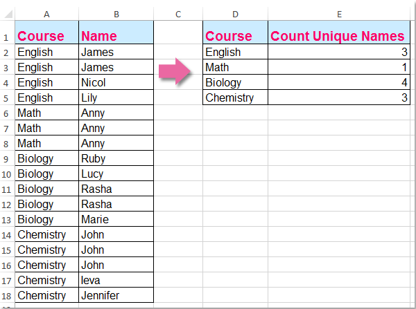
B’fhéidir go mbeadh sé coitianta dúinn luachanna uathúla a chomhaireamh i gcolún amháin, ach, san alt seo, labhróidh mé faoi conas luachanna uathúla a chomhaireamh bunaithe ar cholún eile. Mar shampla, tá an dá shonraí colún seo a leanas agam, anois, ní mór dom na hainmneacha uathúla i gcolún B a chomhaireamh bunaithe ar ábhar cholún A chun an toradh seo a leanas a fháil:

Líon luachanna uathúla bunaithe ar cholún eile le foirmle eagar


mboilgeog cheart gorm saighead Líon luachanna uathúla bunaithe ar cholún eile le foirmle eagar

Chun an fhadhb seo a réiteach, is féidir leis an bhfoirmle seo a leanas cabhrú leat, déan mar a leanas:

1. Iontráil an fhoirmle seo: =SUMPRODUCT((($A$2:$A$18=D2))/COUNTIFS($A$2:$A$18,$A$2:$A$18&"",$B$2:$B$18,$B$2:$B$18&"")) isteach i gcill bhán inar mian leat an toradh a chur, E2, mar shampla. Agus ansin brúigh Ctrl + Shift + Iontráil eochracha le chéile chun an toradh ceart a fháil, féach an scáileán:

comhaireamh uathúil doc de réir critéar 2

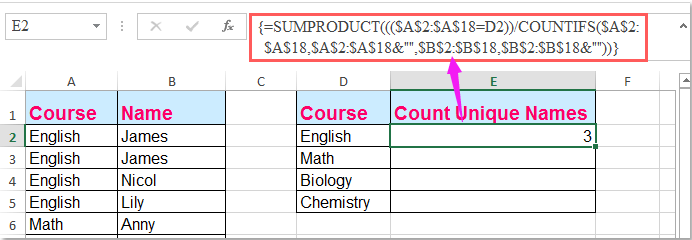
nótaí: San fhoirmle thuas: A2: A18 an bhfuil sonraí na gcolún a ndéanann tú na luachanna uathúla a chomhaireamh bunaithe orthu, B2: B18 an colún ar mhaith leat na luachanna uathúla a chomhaireamh, D2 tá na critéir a chomhaireamh tú uathúil bunaithe ar.

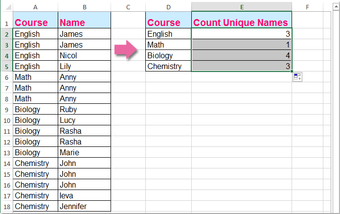
2. Ansin tarraing an láimhseáil líonta síos chun luachanna uathúla na gcritéar comhfhreagrach a fháil. Féach an pictiúr:

comhaireamh uathúil doc de réir critéar 3


Earraí gaolmhara:

Conas líon na luachanna uathúla a chomhaireamh i raon in Excel?

Conas luachanna uathúla a chomhaireamh i gcolún scagtha in Excel?

Conas luachanna céanna nó luachanna dúblacha a chomhaireamh ach uair amháin i gcolún?

Uirlisí Táirgiúlachta Oifige is Fearr

🤖 Kutools AI Aide: anailís sonraí a réabhlóidiú bunaithe ar: Forghníomhú Chliste   |  Gin Cód  |  Cruthaigh Foirmlí Saincheaptha  |  Anailís a dhéanamh ar Sonraí agus Cairteacha a Ghin  |  Feidhmeanna Kutools a agairt...
Gnéithe Coitianta: Faigh, Aibhsigh nó Aithnigh Dúblaigh   |  Scrios Sraitheanna Bána   |  Comhcheangail Colúin nó Cealla gan Sonraí a Chailleadh   |   Babhta gan Foirmle ...
Cuardaigh Super: Ilchritéir VLookup    VLookup Illuachanna  |   VLookup Trasna Ilbhileoga   |   Amharc doiléir ....
Liosta anuas Casta: Go tapa Cruthaigh Liosta Anuas   |  Liosta anuas Cleithiúnach   |  Liosta Buail Isteach Ilroghnacha ....
Bainisteoir Colún: Cuir Líon Sonrach Colún leis  |  Colúin Bog  |  Scoránaigh Stádas Infheictheachta na gColún Ceilte  |  Déan comparáid idir Raonta & Colúin ...
Gnéithe Réadmhaoin: Fócas Eangaí   |  Amharc Dearaidh   |   Barra Mór na Foirmle    Leabhar Oibre & Bainisteoir Bileog   |  Leabharlann Acmhainní (Uaththéacs)   |  Piocálaí Dáta   |  Comhcheangail Bileoga Oibre   |  Criptigh/Díchriptigh Cealla    Seol Ríomhphost trí Liosta   |  Scagaire Super   |   Scagaire Speisialta (scagaire trom/iodálach/stailc tríd...) ...
Barr 15 Uirlisí12 Téacs uirlisí (Cuir Téacs, Bain Carachtair,...)   |   50 + Cairt cineálacha (Cairt Gantt,...)   |   40+ Praiticiúil Foirmlí (Ríomh aois bunaithe ar lá breithe,...)   |   19 Insertion uirlisí (Cuir isteach Cód QR, Ionsáigh Pictiúr ón gCosán,...)   |   12 Tiontú uirlisí (Uimhreacha le Focail, Comhshó Airgeadra,...)   |   7 Cumaisc & Scoilt uirlisí (Sraitheanna Comhcheangail Casta, Cealla Scoilt,...)   |   ... agus eile

Supercharge Do Scileanna Excel le Kutools le haghaidh Excel, agus Éifeachtúlacht Taithí Cosúil Ná Roimhe. Kutools le haghaidh Excel Tairiscintí Níos mó ná 300 Ardghnéithe chun Táirgiúlacht a Treisiú agus Sábháil Am.  Cliceáil anseo chun an ghné is mó a theastaíonn uait a fháil ...

Tuairisc


Tugann Tab Oifige comhéadan Tabbed chuig Office, agus Déan Do Obair i bhfad Níos Éasca

  • Cumasaigh eagarthóireacht agus léamh tabbed i Word, Excel, PowerPoint, Foilsitheoir, Rochtain, Visio agus Tionscadal.
  • Oscail agus cruthaigh cáipéisí iolracha i gcluaisíní nua den fhuinneog chéanna, seachas i bhfuinneoga nua.
  • Méadaíonn do tháirgiúlacht 50%, agus laghdaíonn sé na céadta cad a tharlaíonn nuair luch duit gach lá!
Comments (20)
No ratings yet. Be the first to rate!
This comment was minimized by the moderator on the site
Hi, thanks for this formula, I'm having an issue implementing it across two Worksheets. In my example, your columns A and B are on one sheet, and D and E are on another, which collects similar data from other year-based Sheets. If I put the formula on the sheet where D (Area) and E are, in E it just returns a zero =SUMPRODUCT(((MHST2324[@Team]=[@Area]))/COUNTIFS(MHST2324[@Team],MHST2324[@Team]&"",MHST2324[@School],MHST2324[@School]&"")). However if I put the formula on the Sheet where A (Team) and B (School) are, it works =SUMPRODUCT((([@Team]=Schools[Area]))/COUNTIFS([@Team],[@Team]&"",[@School],[@School]&"")), any ideas as to why?
This comment was minimized by the moderator on the site
Hey, thanks for this formula, I'm having a problem where
This comment was minimized by the moderator on the site
Классная формула, но как сделать чтобы в столбец A и B можно было постоянно добавлять и не менять формулу ? закрепить не диапазон а столбцы
This comment was minimized by the moderator on the site
Hello, DM,
In fact, you can enlarg the cell references as you need. For example:
=SUMPRODUCT((($A$2:$A$10000=D2))/COUNTIFS($A$2:$A$10000,$A$2:$A$10000&"",$B$2:$B$10000,$B$2:$B$10000&""))
Please remeber to press Ctrl + Shift + Enter keys together.
Please have a try, hope it can help you!
This comment was minimized by the moderator on the site
Is there a way to do this but not count a blank cell as a value?
This comment was minimized by the moderator on the site
Hello, MB
To count the unqiue values with criteria and skip the blank cell, you should apply the below array formula:
=SUM(--(FREQUENCY(IF($B$2:$B$15<>"",IF($A$2:$A$15=D2,MATCH($B$2:$B$15,$B$2:$B$15,0))),ROW($B$2:$B$15)-ROW(B2)+1)>0))


After pasting the fromula, please press Ctrl + Shift + Enter keys together.

https://www.extendoffice.com/images/stories/comments/comment-skyyang/doc-count-unique-criteria.png

Please try, hope it can help you!
This comment was minimized by the moderator on the site
Thank you very much for this but how does it work with a large data set. I realised it returns #N/A when the data is beyond row 78
This comment was minimized by the moderator on the site
I would need to do something similar but with dates: on a sheet in which the dates are indicated in the first column, many repeated, I would like to know how many different dates there are that meet a certain condition that appears in another column. I am applying that formula but it gives me an error. Could you help me? Thanks.
This comment was minimized by the moderator on the site
Does anyone know what the ampersand-quotes (" &"" ") in the Criteria 1 and 2 portion of the COUNTIFS formula is doing? This formula worked for me I was just hoping to understand it better.
This comment was minimized by the moderator on the site
Worked like a charm. Very much greatful to you.
This comment was minimized by the moderator on the site
OMG.... I have been searching for over a week for a formula that came close to helping me do a distinct count of one column based on another column.... YOURS FINALLY HELPED ;0) I am so happy!!!!!! Now I just need this formula that you posted to do the same thing but based on 2 column instead of one. I am going to try on my own but do you think you can help?
This comment was minimized by the moderator on the site
Hello, EB, To count the unique values based on two columns, please apply the below formula, after entering the formula, please press Ctrl + Shift + Enter keys together to get the correct result.=SUM(IFERROR(($A$2:$A$15=E2)*($B$2:$B$15=F2)/COUNTIFS($C$2:$C$15,$C$2:$C$15,$A$2:$A$15,E2,$B$2:$B$15,F2),0))
Please try, hope it can help you!
This comment was minimized by the moderator on the site
WOAH, you're a savior, thank you for sharing
This comment was minimized by the moderator on the site
Nevermind it did
There are no comments posted here yet
Load More
Please leave your comments in English
Posting as Guest
×
Rate this post:
0   Characters
Suggested Locations