Conas ach cuid de luach cille a cheilt in Excel?

Má ghlactar leis go bhfuil bileog agat le roinnt faisnéise ginearálta faoin bhfoireann, ach tá cuid acu príobháideach mar uimhreacha slándála sóisialta. Anois is mian leat cuid de na huimhreacha slándála sóisialta seo a cheilt mar atá thíos an pictiúr a thaispeántar, conas is féidir leat iad a réiteach go tapa?

Déan uimhreacha slándála sóisialta a cheilt go páirteach le Cealla Formáid

Déan téacs nó uimhir a cheilt go páirteach le foirmlí

Déan uimhreacha slándála sóisialta a cheilt go páirteach le Cealla Formáid

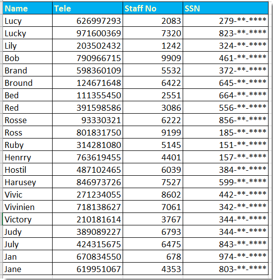
Chun cuid d’uimhreacha slándála sóisialta in Excel a cheilt, is féidir leat Cealla Formáid a chur i bhfeidhm chun iad a réiteach.

1. Roghnaigh na huimhreacha is mian leat a cheilt i bpáirt, agus cliceáil ar dheis chun iad a roghnú Cealla Formáid ón roghchlár comhthéacs. Féach an pictiúr:

2. Ansin sa Cealla Formáid dialóg, cliceáil Uimhir tab, agus roghnaigh An Chustaim ó Catagóir pána, agus téigh chun dul isteach air seo 000 ,, "- ** - ****" isteach sa cineál bosca sa chuid dheis. Féach an pictiúr:

3. cliceáil OK, anois tá na huimhreacha páirteach a roghnaigh tú i bhfolach.

nótaí： Slánóidh sé an uimhir má tá an uimhir amach níos mó ná nó eaqul go 5.

Déan téacs nó uimhir a cheilt go páirteach le foirmlí

Leis an modh thuas, ní féidir leat ach páirtuimhreacha a cheilt, más mian leat páirtuimhreacha nó téacsanna a cheilt, is féidir leat a dhéanamh mar atá thíos:

Folaímid anseo na chéad 4 uimhir d’uimhir an phas.

Roghnaigh cill bhán amháin in aice leis an uimhir phas, F22 mar shampla, iontráil an fhoirmle seo = "****" & CEART (E22,5), agus ansin láimhseáil autofill a tharraingt thar an gcill is gá duit an fhoirmle seo a chur i bhfeidhm.

Leid:

Más mian leat na ceithre uimhir dheireanacha a cheilt, bain úsáid as an bhfoirmle seo, = LEFT (H2,5) & "****"

más mian leat lár-uimhreacha a cheilt, bain úsáid as seo = LEFT (H2,3) & "***" & CEART (H2,3)

Uirlisí Táirgiúlachta Oifige is Fearr

🤖	Kutools AI Aide: anailís sonraí a réabhlóidiú bunaithe ar: Forghníomhú Chliste   |  Gin Cód  |  Cruthaigh Foirmlí Saincheaptha  |  Anailís a dhéanamh ar Sonraí agus Cairteacha a Ghin  |  Feidhmeanna Kutools a agairt...
	Gnéithe Coitianta: Faigh, Aibhsigh nó Aithnigh Dúblaigh   |  Scrios Sraitheanna Bána   |  Comhcheangail Colúin nó Cealla gan Sonraí a Chailleadh   |   Babhta gan Foirmle ...
	Cuardaigh Super: Ilchritéir VLookup  |   VLookup Illuachanna  |   VLookup Trasna Ilbhileoga   |   Amharc doiléir ....
	Liosta anuas Casta: Go tapa Cruthaigh Liosta Anuas   |  Liosta anuas Cleithiúnach   |  Liosta Buail Isteach Ilroghnacha ....
	Bainisteoir Colún: Cuir Líon Sonrach Colún leis  |  Colúin Bog  |  Scoránaigh Stádas Infheictheachta na gColún Ceilte  |  Déan comparáid idir Raonta & Colúin ...
	Gnéithe Réadmhaoin: Fócas Eangaí   |  Amharc Dearaidh   |   Barra Mór na Foirmle   |  Leabhar Oibre & Bainisteoir Bileog   |  Leabharlann Acmhainní (Uaththéacs)   |  Piocálaí Dáta   |  Comhcheangail Bileoga Oibre   |  Criptigh/Díchriptigh Cealla   |  Seol Ríomhphost trí Liosta   |  Scagaire Super   |   Scagaire Speisialta (scagaire trom/iodálach/stailc tríd...) ...
	Barr 15 Uirlisí:  12 Téacs uirlisí (Cuir Téacs, Bain Carachtair,...)   |   50 + Cairt cineálacha (Cairt Gantt,...)   |   40+ Praiticiúil Foirmlí (Ríomh aois bunaithe ar lá breithe,...)   |   19 Insertion uirlisí (Cuir isteach Cód QR, Ionsáigh Pictiúr ón gCosán,...)   |   12 Tiontú uirlisí (Uimhreacha le Focail, Comhshó Airgeadra,...)   |   7 Cumaisc & Scoilt uirlisí (Sraitheanna Comhcheangail Casta, Cealla Scoilt,...)   |   ... agus eile

Supercharge Do Scileanna Excel le Kutools le haghaidh Excel, agus Éifeachtúlacht Taithí Cosúil Ná Roimhe. Kutools le haghaidh Excel Tairiscintí Níos mó ná 300 Ardghnéithe chun Táirgiúlacht a Treisiú agus Sábháil Am.  Cliceáil anseo chun an ghné is mó a theastaíonn uait a fháil ...

Leigh Nios mo... Íoslódáil saor in aisce ...

---

Tugann Tab Oifige comhéadan Tabbed chuig Office, agus Déan Do Obair i bhfad Níos Éasca

• Cumasaigh eagarthóireacht agus léamh tabbed i Word, Excel, PowerPoint, Foilsitheoir, Rochtain, Visio agus Tionscadal.
• Oscail agus cruthaigh cáipéisí iolracha i gcluaisíní nua den fhuinneog chéanna, seachas i bhfuinneoga nua.
• Méadaíonn do tháirgiúlacht 50%, agus laghdaíonn sé na céadta cad a tharlaíonn nuair luch duit gach lá!

Leigh Nios mo... Íoslódáil saor in aisce ...