
Conas an chéad earra ar an liosta anuas a thaispeáint in ionad bán?

doc liosta anuas réamhshocraithe go barr 1

D’fhéadfadh an liosta anuas i mbileog oibre cabhrú linn iontráil sonraí a dhéanamh níos éasca, ní gá dúinn ach na míreanna a roghnú gan iad a chlóscríobh ceann ar cheann. Ach, am éigin, nuair a chliceálann tú an liosta anuas, léimeann sé chuig na míreanna bána ar dtús in ionad na chéad earra sonraí mar a leanas an pictiúr a thaispeántar, d’fhéadfadh sé seo a bheith ina chúis leis na sonraí foinse ag deireadh an liosta a scriosadh. D’fhéadfadh sé a bheith buartha go gcaithfidh tú scrollú ar ais go barr liosta fada do gach cill bhailíochtaithe sonraí bán. An t-alt seo, labhróidh mé faoi conas an chéad earra ar an liosta anuas a thaispeáint i gcónaí.

Taispeáin an chéad earra ar an liosta anuas in ionad bán le feidhm Bailíochtaithe Sonraí

Taispeáin an chéad earra go huathoibríoch ar an liosta anuas in ionad bán le cód VBA


mboilgeog cheart gorm saighead Taispeáin an chéad earra ar an liosta anuas in ionad bán le feidhm Bailíochtaithe Sonraí

I ndáiríre, chun an post seo a bhaint amach, ní gá duit ach foirmle ar leith a chur i bhfeidhm nuair a chruthaíonn tú liosta anuas, déan mar a leanas:

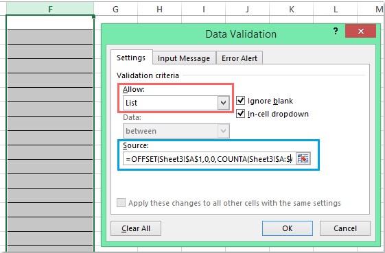
1. Roghnaigh na cealla inar mian leat an liosta anuas a chur isteach, agus cliceáil Dáta > Bailíochtú Sonraí > Bailíochtú Sonraí, féach ar an scáileán:

doc liosta anuas réamhshocraithe go barr 2

2. Sa popped amach Bailíochtú Sonraí bosca dialóige, faoin Socruithe cluaisín, roghnaigh liosta ó na Ceadaigh alt, agus ansin cuir isteach an fhoirmle seo: = OFFSET (Bileog3! $ A $ 1,0,0, COUNTA (Bileog3! $ A: $ A) -1,1) isteach sa Foinse bosca téacs, féach an pictiúr:

nótaí: San fhoirmle seo, Sheet3 an bhfuil an liosta sonraí foinse sa bhileog oibre, agus A1 Is é an chéad luach cille ar an liosta.

doc liosta anuas réamhshocraithe go barr 3

3. Ansin cliceáil OK cnaipe, anois, nuair a chliceálann tú cealla an liosta anuas, an chéad earra sonraí a thaispeántar i gcónaí ag an mbarr cibé an bhfuil luachanna cille scriosta ag deireadh na sonraí foinse, féach an scáileán:

doc liosta anuas réamhshocraithe go barr 4


mboilgeog cheart gorm saighead Taispeáin an chéad earra go huathoibríoch ar an liosta anuas in ionad bán le cód VBA

Anseo, is féidir liom cód VBA a thabhairt isteach a chabhróidh leat an chéad earra ar an liosta anuas a thaispeáint go huathoibríoch nuair a chliceálann tú na cealla bailíochtaithe sonraí.

1. Tar éis duit an liosta anuas a chur isteach, roghnaigh an cluaisín bileog oibre ina bhfuil an liosta anuas, agus cliceáil ar dheis chun é a roghnú Féach an cód ón roghchlár comhthéacs le dul chuig an Microsoft Visual Basic d’Fheidhmchláir fuinneog, agus ansin cóipeáil agus greamaigh an cód seo a leanas sa Mhodúl:

Cód VBA: Taispeáin an chéad mhír sonraí go huathoibríoch ar an liosta anuas:

Private Sub Worksheet_SelectionChange(ByVal Target As Range)
'Updateby Extendoffice 20160725
    Dim xFormula As String
    On Error GoTo Out:
    xFormula = Target.Cells(1).Validation.Formula1
    If Left(xFormula, 1) = "=" Then
        Target.Cells(1) = Range(Mid(xFormula, 1)).Cells(1).Value
    End If
Out:
End Sub

doc liosta anuas réamhshocraithe go barr 5

2. Ansin sábháil agus dún an fhuinneog cód, agus anois, nuair a chliceálann tú cill an liosta anuas, taispeánfar an chéad earra sonraí ag an am céanna.

Uirlisí Táirgiúlachta Oifige is Fearr

🤖 Kutools AI Aide: anailís sonraí a réabhlóidiú bunaithe ar: Forghníomhú Chliste   |  Gin Cód  |  Cruthaigh Foirmlí Saincheaptha  |  Anailís a dhéanamh ar Sonraí agus Cairteacha a Ghin  |  Feidhmeanna Kutools a agairt...
Gnéithe Coitianta: Faigh, Aibhsigh nó Aithnigh Dúblaigh   |  Scrios Sraitheanna Bána   |  Comhcheangail Colúin nó Cealla gan Sonraí a Chailleadh   |   Babhta gan Foirmle ...
Cuardaigh Super: Ilchritéir VLookup    VLookup Illuachanna  |   VLookup Trasna Ilbhileoga   |   Amharc doiléir ....
Liosta anuas Casta: Go tapa Cruthaigh Liosta Anuas   |  Liosta anuas Cleithiúnach   |  Liosta Buail Isteach Ilroghnacha ....
Bainisteoir Colún: Cuir Líon Sonrach Colún leis  |  Colúin Bog  |  Scoránaigh Stádas Infheictheachta na gColún Ceilte  |  Déan comparáid idir Raonta & Colúin ...
Gnéithe Réadmhaoin: Fócas Eangaí   |  Amharc Dearaidh   |   Barra Mór na Foirmle    Leabhar Oibre & Bainisteoir Bileog   |  Leabharlann Acmhainní (Uaththéacs)   |  Piocálaí Dáta   |  Comhcheangail Bileoga Oibre   |  Criptigh/Díchriptigh Cealla    Seol Ríomhphost trí Liosta   |  Scagaire Super   |   Scagaire Speisialta (scagaire trom/iodálach/stailc tríd...) ...
Barr 15 Uirlisí12 Téacs uirlisí (Cuir Téacs, Bain Carachtair,...)   |   50 + Cairt cineálacha (Cairt Gantt,...)   |   40+ Praiticiúil Foirmlí (Ríomh aois bunaithe ar lá breithe,...)   |   19 Insertion uirlisí (Cuir isteach Cód QR, Ionsáigh Pictiúr ón gCosán,...)   |   12 Tiontú uirlisí (Uimhreacha le Focail, Comhshó Airgeadra,...)   |   7 Cumaisc & Scoilt uirlisí (Sraitheanna Comhcheangail Casta, Cealla Scoilt,...)   |   ... agus eile

Supercharge Do Scileanna Excel le Kutools le haghaidh Excel, agus Éifeachtúlacht Taithí Cosúil Ná Roimhe. Kutools le haghaidh Excel Tairiscintí Níos mó ná 300 Ardghnéithe chun Táirgiúlacht a Treisiú agus Sábháil Am.  Cliceáil anseo chun an ghné is mó a theastaíonn uait a fháil ...

Tuairisc


Tugann Tab Oifige comhéadan Tabbed chuig Office, agus Déan Do Obair i bhfad Níos Éasca

  • Cumasaigh eagarthóireacht agus léamh tabbed i Word, Excel, PowerPoint, Foilsitheoir, Rochtain, Visio agus Tionscadal.
  • Oscail agus cruthaigh cáipéisí iolracha i gcluaisíní nua den fhuinneog chéanna, seachas i bhfuinneoga nua.
  • Méadaíonn do tháirgiúlacht 50%, agus laghdaíonn sé na céadta cad a tharlaíonn nuair luch duit gach lá!
Comments (10)
No ratings yet. Be the first to rate!
This comment was minimized by the moderator on the site
=OFFSET(Sheet3!$A$1,0,0,COUNTA(Sheet3!$A:$A)+2-1,1) I added +2 to the equation and that worked for me.
This comment was minimized by the moderator on the site
For the VDA code, how can I have only a certain cell range show the first item in the drop down list? Thank you in advance.
This comment was minimized by the moderator on the site
Hi, Akrupa,To solve your problem, maybe the following VBA code can help you:

<div data-tag="code">Private Sub Worksheet_SelectionChange(ByVal Target As Range)
'Updateby Extendoffice 20211206
Dim xFormula As String
Dim xRg As Range
Dim xStr As String
Dim xIndex As Integer
xIndex = 2 'Here indicates the cell number of the original data,for example,the original data is A1:A10, to display the A2 cell value, please write 2 here.
On Error GoTo Out:
xFormula = Target.Cells(1).Validation.Formula1
If Left(xFormula, 1) = "=" Then
If Target.Value <> "" Then Exit Sub
xStr = Mid(xFormula, 2)
Set xRg = Application.Range(xStr)
Target.Cells(1) = xRg.Cells(xIndex).Value
End If
Out:
End Sub
Please try, hope it can help you!
This comment was minimized by the moderator on the site
Better but not quite. Using the =OFFSET(Sheet3!$A$1,0,0,COUNTA(Sheet3!$A:$A)-1,1) method eliminates the blanks but still starts you at the bottom of the very long list. I want it to start at the top of the list.
This comment was minimized by the moderator on the site
Once again, you save the day! Thanks!
This comment was minimized by the moderator on the site
Doesn't work for me. I keep getting an error message that says, "There's a problem with this formula. Not trying to type a formula? When the first character is an equal (+) or minus (-) sign, Exel thinks it's a formula.... To get around this, type an apostrophe (') first..."
This comment was minimized by the moderator on the site
Hello!

How can I set a data validation list such that if the drop down value in the cell is deleted, the cell will automatically show a default value (i.e. "-Select-")?

For example, I have a worksheet with multiple drop down lists that I want to show a default value of "-Select-" once the sheet is opened. A user will select values from the lists that will impact the result of calculations throughout the entire spreadsheet. A user may accidentally "delete" the cell contents of the lists. If this happens, rather than the cell becoming blank, I want the cell to show a default value of "-Select-". This scenario occurs in multiple random locations throughout the spreadsheet, not just in one localized place.

I was able to find the following VBA code so far, but it only applies the concept over a range, rather than just individual cells that contain drop down lists. The problem with what I have coded so far is that every single blank cell in the range ends up with "-Select-" in it. Some of the lists are in ranges, but some are also scattered throughout the sheet. The problem I'm having with my current code is that every single blank cell in the range ends up with "-Select-" in it. I'm trying to get this to apply over the entire worksheet to ONLY cells that are drop down lists.

Is what I'm trying to accomplish even possible?

Example file can be found here:
https://drive.google.com/file/d/1VoO8VgFs3IJ0ALwqfk0i8gt69UE4vEKW/view?usp=sharing

Example code:

Option Explicit

Private Sub Worksheet_Change(ByVal Target As Range)
Dim cel As Range
' If Target.Cells.Count > 1 Then Exit Sub 'turning this off allows multiple cells to be selected and deleted at the same time
If Not Intersect(Target, Range("f2:p17")) Is Nothing Then
For Each cel In Range("f2:p17")
Application.EnableEvents = False
If IsEmpty(cel.Value) Then cel.Value = "-Select-"
Next cel
End If
Application.EnableEvents = True
End Sub


Thanks in advance!
This comment was minimized by the moderator on the site
How can I set a data validation list such that if the drop down value in the cell is deleted, the cell will automatically show the a default value (i.e. "-Select-")?

For example, I have a worksheet with multiple drop down lists that I want to show a default value of "-Select-" once the sheet is opened. A user will select values from the lists that will impact the result of calculations throughout the entire spreadsheet. A user may accidentally "delete" the cell contents. If this happens, rather than the cell becoming blank, I want the cell to show a default value of "-Select-". This scenario occurs in multiple random locations throughout the spreadsheet, not just in one localized place.

I was able to come up with the following VBA code so far, but I've only figured out how to apply the concept over a range, rather than just cells that contain a drop down list. The problem with what I have coded so far is that every single blank cell in the range ends up with "-Select-" in it.

Option Explicit

Private Sub Worksheet_Change(ByVal Target As Range)
Dim cel As Range
' If Target.Cells.Count > 1 Then Exit Sub
If Not Intersect(Target, Range("f2:p17")) Is Nothing Then
For Each cel In Range("f2:p17")
Application.EnableEvents = False
If IsEmpty(cel.Value) Then cel.Value = "-Select-"
Next cel
End If
Application.EnableEvents = True
End Sub
This comment was minimized by the moderator on the site
select the cell in which you have put the listitem
the range for the listitem is "Opleiding"
in your VBA code:

selection.Value = Range("opleiding").Cells(2, 1)

the result is that the selected item of the listItem is the second item in the range "Opleiding"
This comment was minimized by the moderator on the site
After scroll down select to cells numeric data not come in series only first cell data come select 1,2 different cells and scroll down value not coming 1,2,3,4,5....... only first cell value coming 1,1,1,1,....
There are no comments posted here yet
Please leave your comments in English
Posting as Guest
×
Rate this post:
0   Characters
Suggested Locations