
Conas an naoú cill neamh bán a fháil in Excel?

Conas a d’fhéadfá an naoú luach cille neamh bán a fháil agus a thabhairt ar ais ó cholún nó as a chéile in Excel? An t-alt seo, labhróidh mé faoi roinnt foirmlí úsáideacha chun an tasc seo a réiteach.

Faigh agus faigh ar ais an naoú luach cille neamh bán ó cholún le foirmle

Faigh agus seol an naoú luach cille neamh bán as a chéile le foirmle


mboilgeog cheart gorm saighead Faigh agus faigh ar ais an naoú luach cille neamh bán ó cholún le foirmle

Mar shampla, tá colún sonraí agam mar a leanas an pictiúr a thaispeántar, anois, gheobhaidh mé an tríú luach cille neamh bán ón liosta seo.

faigh nth neamh bán 1

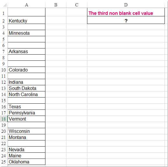
Iontráil an fhoirmle seo le do thoil: =INDEX($A$1:$A$25,SMALL(ROW($A$1:$A$25)+(100*($A$1:$A$25="")), 3))&"" isteach i gcill bhán inar mian leat an toradh, D2, a aschur, mar shampla, agus ansin brúigh Ctrl + Shift + Iontráil eochracha le chéile chun an toradh ceart a fháil, féach an scáileán:

faigh nth neamh bán 2

nótaí: San fhoirmle thuas, A1: A25 an liosta sonraí is mian leat a úsáid, agus an uimhir 3 léiríonn sé an tríú luach cille neamh-bán a theastaíonn uait a thabhairt ar ais, más mian leat an dara cill neamh bán a fháil, ní gá duit ach an uimhir 3 go 2 a athrú de réir mar a theastaíonn uait.


mboilgeog cheart gorm saighead Faigh agus seol an naoú luach cille neamh bán as a chéile le foirmle

Más mian leat an naoú luach cille neamh bán a fháil agus a thabhairt ar ais i ndiaidh a chéile, d’fhéadfadh an fhoirmle seo a leanas cabhrú leat, déan mar seo le do thoil:

Iontráil an fhoirmle seo: =INDEX($A$1:$M$1,SMALL(IF($A$1:$M$1<>"",COLUMN($A$1:$M$1)-COLUMN($A$1)+1),4)) isteach i gcill bhán inar mian leat an toradh a aimsiú, agus ansin brúigh Ctrl + Shift + Iontráil eochracha le chéile chun an toradh a fháil, féach an scáileán:

faigh nth neamh bán 3

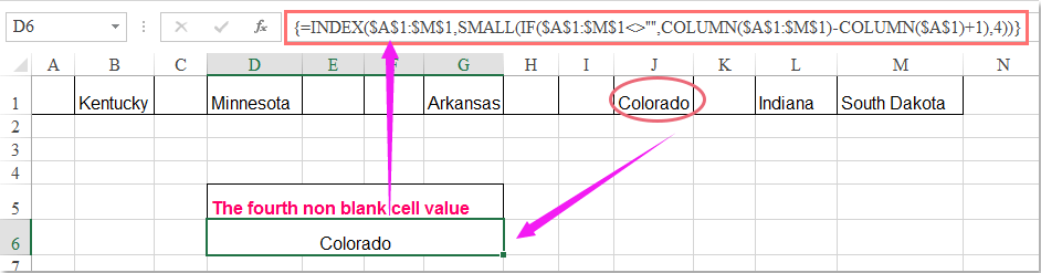
Nóta: San fhoirmle thuas, A1: M1 is iad na luachanna as a chéile a theastaíonn uait a úsáid, agus an uimhir 4 Is é seo an ceathrú luach cille neamh bán a theastaíonn uait a thabhairt ar ais, más mian leat an dara cill neamh bán a fháil, ní gá duit ach an uimhir 4 go 2 a athrú de réir mar a theastaíonn uait.

Uirlisí Táirgiúlachta Oifige is Fearr

🤖 Kutools AI Aide: anailís sonraí a réabhlóidiú bunaithe ar: Forghníomhú Chliste   |  Gin Cód  |  Cruthaigh Foirmlí Saincheaptha  |  Anailís a dhéanamh ar Sonraí agus Cairteacha a Ghin  |  Feidhmeanna Kutools a agairt...
Gnéithe Coitianta: Faigh, Aibhsigh nó Aithnigh Dúblaigh   |  Scrios Sraitheanna Bána   |  Comhcheangail Colúin nó Cealla gan Sonraí a Chailleadh   |   Babhta gan Foirmle ...
Cuardaigh Super: Ilchritéir VLookup    VLookup Illuachanna  |   VLookup Trasna Ilbhileoga   |   Amharc doiléir ....
Liosta anuas Casta: Go tapa Cruthaigh Liosta Anuas   |  Liosta anuas Cleithiúnach   |  Liosta Buail Isteach Ilroghnacha ....
Bainisteoir Colún: Cuir Líon Sonrach Colún leis  |  Colúin Bog  |  Scoránaigh Stádas Infheictheachta na gColún Ceilte  |  Déan comparáid idir Raonta & Colúin ...
Gnéithe Réadmhaoin: Fócas Eangaí   |  Amharc Dearaidh   |   Barra Mór na Foirmle    Leabhar Oibre & Bainisteoir Bileog   |  Leabharlann Acmhainní (Uaththéacs)   |  Piocálaí Dáta   |  Comhcheangail Bileoga Oibre   |  Criptigh/Díchriptigh Cealla    Seol Ríomhphost trí Liosta   |  Scagaire Super   |   Scagaire Speisialta (scagaire trom/iodálach/stailc tríd...) ...
Barr 15 Uirlisí12 Téacs uirlisí (Cuir Téacs, Bain Carachtair,...)   |   50 + Cairt cineálacha (Cairt Gantt,...)   |   40+ Praiticiúil Foirmlí (Ríomh aois bunaithe ar lá breithe,...)   |   19 Insertion uirlisí (Cuir isteach Cód QR, Ionsáigh Pictiúr ón gCosán,...)   |   12 Tiontú uirlisí (Uimhreacha le Focail, Comhshó Airgeadra,...)   |   7 Cumaisc & Scoilt uirlisí (Sraitheanna Comhcheangail Casta, Cealla Scoilt,...)   |   ... agus eile

Supercharge Do Scileanna Excel le Kutools le haghaidh Excel, agus Éifeachtúlacht Taithí Cosúil Ná Roimhe. Kutools le haghaidh Excel Tairiscintí Níos mó ná 300 Ardghnéithe chun Táirgiúlacht a Treisiú agus Sábháil Am.  Cliceáil anseo chun an ghné is mó a theastaíonn uait a fháil ...

Tuairisc


Tugann Tab Oifige comhéadan Tabbed chuig Office, agus Déan Do Obair i bhfad Níos Éasca

  • Cumasaigh eagarthóireacht agus léamh tabbed i Word, Excel, PowerPoint, Foilsitheoir, Rochtain, Visio agus Tionscadal.
  • Oscail agus cruthaigh cáipéisí iolracha i gcluaisíní nua den fhuinneog chéanna, seachas i bhfuinneoga nua.
  • Méadaíonn do tháirgiúlacht 50%, agus laghdaíonn sé na céadta cad a tharlaíonn nuair luch duit gach lá!
Comments (10)
No ratings yet. Be the first to rate!
This comment was minimized by the moderator on the site
CIAO STO CERCANDO DI APPLICARE LA TUA FORMULA MA NON MI FUNZIONA, DOVE STO SBAGLIANDO?
=INDICE($K$37:$K$88;MIN(RIGHE($K$37:$K$88)+RIGHE(100*($K$37:$K$88=""));6))&""
DEVO VISUALIZZARE L'ENNESIMA RIGA DIVERSA DA VUOTO

GRAzie
This comment was minimized by the moderator on the site
=INDICE($K$37:$K$88;MIN(RIGHE($K$37:$K$88)+(100*($K$37:$K$88=""));6))&""
This comment was minimized by the moderator on the site
I'm running this formula on a ~400 row sheet with around 20 blanks mixed throughout the data, and it's working perfectly EXCEPT when I fill the series down, it sometimes duplicates a row for some reason. For example, it seems to think a value is somehow simultaneously the 331st non-blank and the 332nd.

Things I've noticed:
-Duplications always happen in pairs (ex. 331 and 332 are duplicates, 333 and 334 will also be), then it goes back to normal for a while.
-Raw data also has blanks in pairs, but not corresponding to the duplicates
-No duplications occur in the first 94 rows, but they happen every 33-35 rows after that
-Does not appear to be linked to the value in the cell being duplicated
-I have entered as an array and as a standard formula, no difference in function

For reference, here's my actual formula:

=INDEX('PO Raw Data'!CR:CR,SMALL(ROW('PO Raw Data'!CR:CR)+(100*('PO Raw Data'!CR:CR="")),$W2)&"")

Note $W2 refers to a helper column and counts up as the data set is filled down, but only because I couldn't get it to count up when I just used a number instead of cell reference.
When I've replaced that cell reference (ex. $W2) with the appropriate number, same result.


Any thoughts on what I can do to fix that?
This comment was minimized by the moderator on the site
very helpful,
although when I return the nth non blank cell in a column set to DATE, the returned value appears as number(general number).formatting the cell into DATE also doesn't change the result. could you please give me a hand!
thanks a lot
This comment was minimized by the moderator on the site
Hello, Shirazi,
Sorry, maybe there is no direct formula for you to get the date format.

If someone else has the solution, please comment here.
This comment was minimized by the moderator on the site
Hi everyone!


Could you also help me return the row number of the second, third non-blank cell?


Please help me.
This comment was minimized by the moderator on the site
Hello, John,
the following formula can help you to get all the row numbers of the non-blank cells, please try it, thank you!
=IFERROR(ROW(INDEX($A$1:$A$12,SMALL(INDEX(NOT(ISBLANK($A$1:$A$12))*ROW($A$1:$A$12),0),COUNTBLANK($A$1:$A$12)+ROW(A1)))),"")
This comment was minimized by the moderator on the site
Hey everyone,

I have a table with numerous columns and rows. The rows have range names, and a description/location at the beginning of the row range with its own range, example "Building No.s". There are multiple Row Ranges/ Buildings. There are headers at the top of each columns for specific "Building Assembly Types". The table content is numeric quantities for each type "Building Assembly Type" for each specific "Building" description/location. There could be as many as (100) "Building Assembly Types" column headers but I will limit the assemblies to (10) per row range, so there will be numerous blank cells in each "Building No." range.

I have other summary tables set up for each "Building" that I want to pull the non-blank cells quantities to, along with the corresponding header "Assembly Type" for each "Building" with a (10) max "Assemblies" per page.

I can identify the non-blank cell quantities by use of the array formula above for rows. The problem I am having is identifying the header that corresponds to it.

Ultimately if I can identify the "Assembly" header, I can always index the "Quantities" once I have the header "Assembly" identified for each "Building". Then I would be able do a lookup for all the parts associated with each "Assembly" type for that "Building" from my Assembly parts database and multiply it times the "Quantity" of each assembly type.

Hopefully this makes since and someone can help.
This comment was minimized by the moderator on the site
Hello, I am looking for the third blank row in a column and I copied your formula and just changed the range from $A$1:$A:$25 to my range $D$306:$D$354. But when I change the range I get #REF! as my answer. I already converted to an array, control-shift-enter. Now the cell range I am referencing has formulas in them, so could that be why I am getting #REF. Your formula: =INDEX($A$1:$A$25,SMALL(ROW($A$1:$A$25)+(100*($A$1:$A$25="")), 3))&"" My formula: =INDEX($D$306:$D$354,SMALL(ROW($D$306:$D$354)+(1*($D$306:$D$354="")), 2))&"" Thanks, Noel
This comment was minimized by the moderator on the site
you have put the 1 instead of 100 therefore answered was wrong. please use below formula

INDEX($D$306:$D$354,SMALL(ROW($D$306:$D$354)+(100*($D$306:$D$354="")), 3))&"" than ctrl + shift+enter
There are no comments posted here yet
Please leave your comments in English
Posting as Guest
×
Rate this post:
0   Characters
Suggested Locations