
Conas do bhosca cuardaigh féin a chruthú in Excel?

Seachas an fheidhm Aimsigh in Excel a úsáid, i ndáiríre is féidir leat do bhosca cuardaigh féin a chruthú chun na luachanna riachtanacha a chuardach go héasca. Taispeánfaidh an t-alt seo dhá mhodh duit chun do bhosca cuardaigh féin a chruthú in Excel go mion.

Cruthaigh do bhosca cuardaigh féin le Formáidiú Coinníollach chun aird a tharraingt ar gach toradh a ndearnadh cuardach air
Cruthaigh do bhosca cuardaigh féin le foirmlí chun na torthaí cuardaigh go léir a liostáil


Cruthaigh do bhosca cuardaigh féin le Formáidiú Coinníollach chun aird a tharraingt ar gach toradh a ndearnadh cuardach air

Is féidir leat é seo a leanas a dhéanamh chun do bhosca cuardaigh féin a chruthú tríd an bhfeidhm Formáidithe Coinníollach a úsáid in Excel.

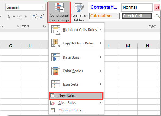
1. Roghnaigh an raon le sonraí a theastaíonn uait a chuardach sa bhosca cuardaigh, ansin cliceáil Formáidiú Coinníollach > Riail Nua faoi ​​na Baile cluaisín. Féach an pictiúr:

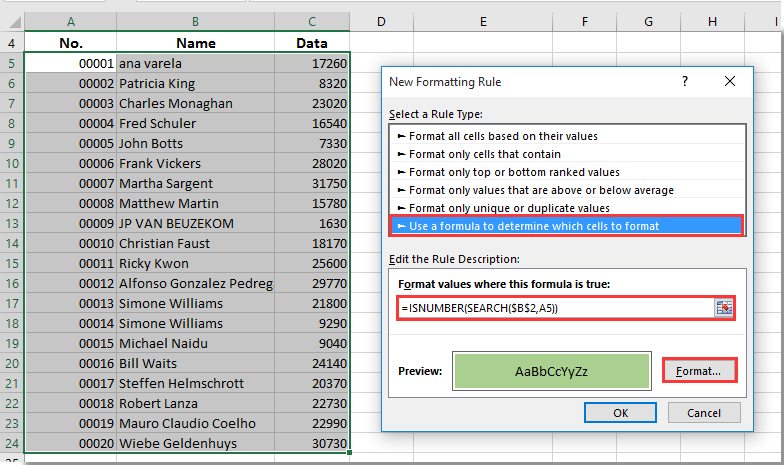
2. Sa Riail Nua Formáidithe bosca dialóige, ní mór duit:

2.1) Roghnaigh Úsáid foirmle chun a fháil amach cé na cealla atá le formáidiú rogha sa Roghnaigh Cineál Riail bosca;

2.2) Iontráil foirmle = ISNUMBER (CUARDACH ($ B $ 2, A5)) isteach sa Luachanna formáide nuair atá an fhoirmle seo fíor bosca;

2.3) Cliceáil ar an déanta cnaipe chun dath aibhsithe a shonrú don luach cuardaigh;

2.4) Cliceáil ar an OK cnaipe.

nótaí:

1. San fhoirmle, is cill bán í $ B $ 2 a chaithfidh tú a úsáid mar bhosca cuardaigh, agus is é A5 an chéad chill de do raon roghnaithe a gcaithfidh tú luachanna a chuardach laistigh de. Athraigh iad de réir mar is gá duit.

2. Níl an fhoirmle cás-íogair.

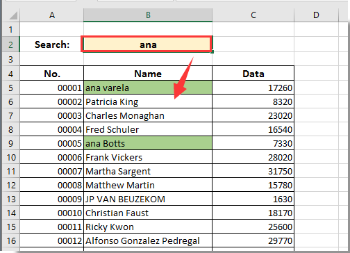
Anois cruthaítear an bosca cuardaigh, agus critéir chuardaigh á gclóscríobh isteach sa bhosca cuardaigh B2 agus brúigh an eochair Iontráil, déantar gach luach comhoiriúnaithe sa raon sonraithe a chuardach agus a aibhsiú láithreach mar a thaispeántar thíos an scáileán.


Cruthaigh do bhosca cuardaigh féin le foirmlí chun na torthaí cuardaigh go léir a liostáil

Má cheaptar go bhfuil liosta sonraí agat atá suite i raon E4: E23 a chaithfidh tú a chuardach, más mian leat na luachanna comhoiriúnaithe go léir a liostáil i gcolún eile tar éis duit cuardach a dhéanamh le do bhosca cuardaigh féin, is féidir leat an modh thíos a thriail.

1. Roghnaigh cill bhán atá cóngarach do chill E4, roghnaigh mé cill D4 anseo, ansin cuir isteach an fhoirmle = IFERROR (CUARDACH ($ B $ 2, E4) + ROW () / 100000, "") isteach sa bharra foirmle, agus ansin brúigh an Iontráil eochair. Féach an pictiúr:

nótaí: San fhoirmle, is é $ B $ 2 an chill a theastaíonn uait a úsáid mar bhosca cuardaigh, is é E4 an chéad chill den liosta sonraí a chaithfidh tú a chuardach. Is féidir leat iad a athrú de réir mar is gá duit.

2. Coinnigh ag roghnú cill E4, ansin tarraing an Láimhseáil Líon isteach go cill D23. Féach an pictiúr:

3. Anois roghnaigh cill C4, cuir isteach an fhoirmle = IFERROR (RANK (D4, $ D $ 4: $ D $ 23,1), "") isteach sa Bharra Foirmle, agus brúigh an Iontráil eochair. Roghnaigh cill C4, ansin tarraing an Láimhseáil Líon isteach go C23. Féach an pictiúr:

4. Anois ní mór duit raon A4: A23 a líonadh le huimhir na sraithe a mhéadaíonn 1 ó 1 go 20 mar atá thíos ar an scáileán:

5. Roghnaigh cill bhán a theastaíonn uait chun an toradh cuardaigh a thaispeáint, cuir isteach an fhoirmle = IFERROR (VLOOKUP (A4, $ C $ 4: $ E $ 23,3, BRÉAGACH), "") isteach sa Bharra Foirmle agus brúigh an Iontráil eochair. Coinnigh ag roghnú cill B4, tarraing an Láimhseáil Líon isteach go B23 mar atá thíos an pictiúr a thaispeántar.

As seo amach, agus sonraí á n-iontráil i mbosca cuardaigh B2, liostófar na luachanna comhoiriúnaithe go léir i raon B4: B23 mar a thaispeántar thíos an pictiúr.

nótaí: níl an modh seo cás-íogair.

Uirlisí Táirgiúlachta Oifige is Fearr

🤖 Kutools AI Aide: anailís sonraí a réabhlóidiú bunaithe ar: Forghníomhú Chliste   |  Gin Cód  |  Cruthaigh Foirmlí Saincheaptha  |  Anailís a dhéanamh ar Sonraí agus Cairteacha a Ghin  |  Feidhmeanna Kutools a agairt...
Gnéithe Coitianta: Faigh, Aibhsigh nó Aithnigh Dúblaigh   |  Scrios Sraitheanna Bána   |  Comhcheangail Colúin nó Cealla gan Sonraí a Chailleadh   |   Babhta gan Foirmle ...
Cuardaigh Super: Ilchritéir VLookup    VLookup Illuachanna  |   VLookup Trasna Ilbhileoga   |   Amharc doiléir ....
Liosta anuas Casta: Go tapa Cruthaigh Liosta Anuas   |  Liosta anuas Cleithiúnach   |  Liosta Buail Isteach Ilroghnacha ....
Bainisteoir Colún: Cuir Líon Sonrach Colún leis  |  Colúin Bog  |  Scoránaigh Stádas Infheictheachta na gColún Ceilte  |  Déan comparáid idir Raonta & Colúin ...
Gnéithe Réadmhaoin: Fócas Eangaí   |  Amharc Dearaidh   |   Barra Mór na Foirmle    Leabhar Oibre & Bainisteoir Bileog   |  Leabharlann Acmhainní (Uaththéacs)   |  Piocálaí Dáta   |  Comhcheangail Bileoga Oibre   |  Criptigh/Díchriptigh Cealla    Seol Ríomhphost trí Liosta   |  Scagaire Super   |   Scagaire Speisialta (scagaire trom/iodálach/stailc tríd...) ...
Barr 15 Uirlisí12 Téacs uirlisí (Cuir Téacs, Bain Carachtair,...)   |   50 + Cairt cineálacha (Cairt Gantt,...)   |   40+ Praiticiúil Foirmlí (Ríomh aois bunaithe ar lá breithe,...)   |   19 Insertion uirlisí (Cuir isteach Cód QR, Ionsáigh Pictiúr ón gCosán,...)   |   12 Tiontú uirlisí (Uimhreacha le Focail, Comhshó Airgeadra,...)   |   7 Cumaisc & Scoilt uirlisí (Sraitheanna Comhcheangail Casta, Cealla Scoilt,...)   |   ... agus eile

Supercharge Do Scileanna Excel le Kutools le haghaidh Excel, agus Éifeachtúlacht Taithí Cosúil Ná Roimhe. Kutools le haghaidh Excel Tairiscintí Níos mó ná 300 Ardghnéithe chun Táirgiúlacht a Treisiú agus Sábháil Am.  Cliceáil anseo chun an ghné is mó a theastaíonn uait a fháil ...

Tuairisc


Tugann Tab Oifige comhéadan Tabbed chuig Office, agus Déan Do Obair i bhfad Níos Éasca

  • Cumasaigh eagarthóireacht agus léamh tabbed i Word, Excel, PowerPoint, Foilsitheoir, Rochtain, Visio agus Tionscadal.
  • Oscail agus cruthaigh cáipéisí iolracha i gcluaisíní nua den fhuinneog chéanna, seachas i bhfuinneoga nua.
  • Méadaíonn do tháirgiúlacht 50%, agus laghdaíonn sé na céadta cad a tharlaíonn nuair luch duit gach lá!
Comments (29)
No ratings yet. Be the first to rate!
This comment was minimized by the moderator on the site
me pueden apoyar en cual es la formula para solo buscar
porfa
This comment was minimized by the moderator on the site
Hi, for the second part: "Create Your Own Search Box With Formulas To List All Searched Results", it doesn't say what to do with the search box, my search box has no formula in it. I am trying to do it with multiple columns as well, does it work too?
This comment was minimized by the moderator on the site
Insert data from example. Copy formula in indicated cell, but delete space from formula. Easy!
This comment was minimized by the moderator on the site
i have tried using this but is dose not wont to highlight the box I am searching for why is this
This comment was minimized by the moderator on the site
Can you create a formula that captures two cells worth of information in retrospect i am using a set up that captures user names and badge data so i need it to when it filters that it carries both cells of information not just one
This comment was minimized by the moderator on the site
hi! I used the basic highlight search bar, but am having a couple of issues. it is predicting my search and finding it with no issues... however, it always highlights the cell a couple below or above the searched one. Are you able to help me with this please?
This comment was minimized by the moderator on the site
Hi! Is this applicable to Google Sheets? I'm trying to make a search box with formulas to list all searched results. I followed every steps listed above but the results shows nothing. There is an error tho, it says "change Iterative calculation". But whatever I do, it doesn't show anything - just blank. Can you help me with this, please... Thank you!
This comment was minimized by the moderator on the site
Good day,
This is only applicable to Microsoft Excel application. Sorry for the inconvenience.
This comment was minimized by the moderator on the site
Hi! Is this applicable to Google Sheets? I'm trying to make a search box with formulas to list all searched results. I followed every steps listed above but the results shows nothing. There is an error tho, it says "change Iterative calculation". But whatever I do, it doesn't show anything - just blank. Can you help me with this, please... Thank you!
This comment was minimized by the moderator on the site
Hello, I am using to search between my vendors (one column) and brands (another column). With this setup, there are brands (like Microsoft) that can have more vendors (vendor A, vendor B, vendor C,...). I would like to search for the brand (microsoft) name and would like to see all possible vendors (A, B & C as well). But now the result is only the first vendor and that's all. How can I change/fix that?

Many thanks!
This comment was minimized by the moderator on the site
Hi Tomas,
Maybe you can rearrange your data and create a dynamic drop down list to solve the problem. You can browse the below article for more details.
https://www.extendoffice.com/documents/excel/1350-excel-create-dynamic-drop-down-list.html
This comment was minimized by the moderator on the site
i followed the resulted search method and it worked perfectly however the results are hyperlinked and it shows me the result without the hyperlink is there a way i can make it show me the result with the link connection?
This comment was minimized by the moderator on the site
After entering the formula =ISNUMBER(SEARCH($B$1,A4)) for conditional formatting, if the cell I used for the search function is blank, all the cells that are searched (A4:C368) are highlighted. But once a string is entered for the search criteria the cells containing the search criteria are highlighted correctly. Is there a way to tweak the formula to not highlight until search criteria is entered? Or did I do something wrong?

Also, using the formula in step 5 on another sheet within the workbook isn't working. What I'm trying to do is perform a search and show results of that search on one sheet named Search & Results while having the information to be searched on a sheet named Index. The formula I'm using is =IFERROR(VLOOKUP(A3,Index!$A$4:$C$368,5,FALSE),"") where A3 is the beginning of my numbered cells on the Search & Results sheet and the search is taking place throughout cells A4:C368 on the Index sheet.
This comment was minimized by the moderator on the site
same had been having the same issue with the formula,try this in your conditional formatting rule "=AND($I$1<>"",ISNUMBER(SEARCH($I$1,$B4)))", it works for me
I1 is my search box, B4 is first cell of selected range
This comment was minimized by the moderator on the site
Hi Colby. Your vlookup formula=IFERROR(VLOOKUP(A3,Index!$A$4:$C$368,5,FALSE),"") refers to range from A4 to C368 in Sheet name index which have only 3 column but you are entering 5 right after $C$368 which tells the vlookup formula to display value of column 5 which does not exists in your selected range. Fix this and I believe that your problem will be solved.
This comment was minimized by the moderator on the site
I have the same problem. Did you get an answer?
This comment was minimized by the moderator on the site
also me. i have the same problem
There are no comments posted here yet
Load More
Please leave your comments in English
Posting as Guest
×
Rate this post:
0   Characters
Suggested Locations