
 Conas uaslíon na n-uimhreacha dearfacha / diúltacha i ndiaidh a chéile a chomhaireamh in Excel?

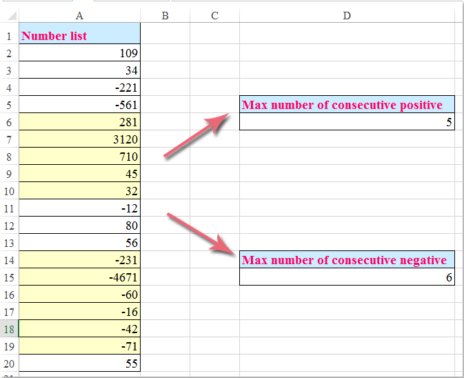
Má tá liosta sonraí agat a mheascann le huimhreacha dearfacha agus diúltacha, agus anois, ba mhaith leat an líon uasta uimhreacha dearfacha agus diúltacha i ndiaidh a chéile a chomhaireamh mar a leanas an pictiúr a thaispeántar, conas a d’fhéadfá déileáil leis an tasc seo in Excel?

Líon na huaslíon uimhreacha dearfacha agus diúltacha i ndiaidh a chéile le foirmlí eagar


Líon na huaslíon uimhreacha dearfacha agus diúltacha i ndiaidh a chéile le foirmlí eagar


Chun an líon uasta uimhreacha dearfacha agus diúltacha i ndiaidh a chéile a fháil, cuir na foirmlí eagar seo a leanas i bhfeidhm:

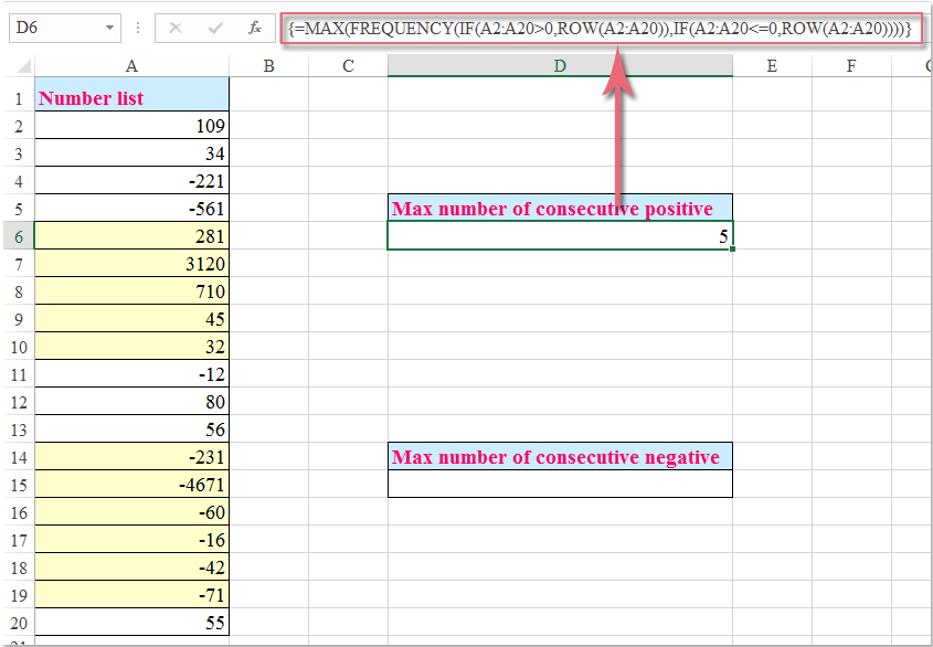
Líon uaslíon na n-uimhreacha dearfacha comhleanúnacha:

Cuir an fhoirmle seo isteach i gcill inar mian leat an toradh a fháil:

=MAX(FREQUENCY(IF(A2:A20>0,ROW(A2:A20)),IF(A2:A20<=0,ROW(A2:A20)))), agus ansin brúigh Ctrl + Shift + Iontráil eochracha le chéile, agus gheobhaidh tú an toradh ceart de réir mar is gá duit, féach an pictiúr:


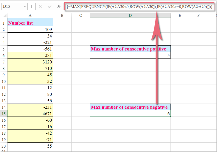
Líon uaslíon na n-uimhreacha diúltacha i ndiaidh a chéile:

Cuir an fhoirmle seo isteach i gcill inar mian leat an toradh a fháil:

=MAX(FREQUENCY(IF(A2:A20<0,ROW(A2:A20)),IF(A2:A20>=0,ROW(A2:A20)))), agus ansin brúigh Ctrl + Shift + Iontráil eochracha ag an am céanna, agus gheobhaidh tú an toradh de réir mar is gá duit, féach an pictiúr:

nótaí: Sna foirmlí thuas, A2: A20 Is é seo liosta na raon cealla is mian leat a úsáid.


Uirlisí Táirgiúlachta Oifige is Fearr

🤖 Kutools AI Aide: anailís sonraí a réabhlóidiú bunaithe ar: Forghníomhú Chliste   |  Gin Cód  |  Cruthaigh Foirmlí Saincheaptha  |  Anailís a dhéanamh ar Sonraí agus Cairteacha a Ghin  |  Feidhmeanna Kutools a agairt...
Gnéithe Coitianta: Faigh, Aibhsigh nó Aithnigh Dúblaigh   |  Scrios Sraitheanna Bána   |  Comhcheangail Colúin nó Cealla gan Sonraí a Chailleadh   |   Babhta gan Foirmle ...
Cuardaigh Super: Ilchritéir VLookup    VLookup Illuachanna  |   VLookup Trasna Ilbhileoga   |   Amharc doiléir ....
Liosta anuas Casta: Go tapa Cruthaigh Liosta Anuas   |  Liosta anuas Cleithiúnach   |  Liosta Buail Isteach Ilroghnacha ....
Bainisteoir Colún: Cuir Líon Sonrach Colún leis  |  Colúin Bog  |  Scoránaigh Stádas Infheictheachta na gColún Ceilte  |  Déan comparáid idir Raonta & Colúin ...
Gnéithe Réadmhaoin: Fócas Eangaí   |  Amharc Dearaidh   |   Barra Mór na Foirmle    Leabhar Oibre & Bainisteoir Bileog   |  Leabharlann Acmhainní (Uaththéacs)   |  Piocálaí Dáta   |  Comhcheangail Bileoga Oibre   |  Criptigh/Díchriptigh Cealla    Seol Ríomhphost trí Liosta   |  Scagaire Super   |   Scagaire Speisialta (scagaire trom/iodálach/stailc tríd...) ...
Barr 15 Uirlisí12 Téacs uirlisí (Cuir Téacs, Bain Carachtair,...)   |   50 + Cairt cineálacha (Cairt Gantt,...)   |   40+ Praiticiúil Foirmlí (Ríomh aois bunaithe ar lá breithe,...)   |   19 Insertion uirlisí (Cuir isteach Cód QR, Ionsáigh Pictiúr ón gCosán,...)   |   12 Tiontú uirlisí (Uimhreacha le Focail, Comhshó Airgeadra,...)   |   7 Cumaisc & Scoilt uirlisí (Sraitheanna Comhcheangail Casta, Cealla Scoilt,...)   |   ... agus eile

Supercharge Do Scileanna Excel le Kutools le haghaidh Excel, agus Éifeachtúlacht Taithí Cosúil Ná Roimhe. Kutools le haghaidh Excel Tairiscintí Níos mó ná 300 Ardghnéithe chun Táirgiúlacht a Treisiú agus Sábháil Am.  Cliceáil anseo chun an ghné is mó a theastaíonn uait a fháil ...

Tuairisc


Tugann Tab Oifige comhéadan Tabbed chuig Office, agus Déan Do Obair i bhfad Níos Éasca

  • Cumasaigh eagarthóireacht agus léamh tabbed i Word, Excel, PowerPoint, Foilsitheoir, Rochtain, Visio agus Tionscadal.
  • Oscail agus cruthaigh cáipéisí iolracha i gcluaisíní nua den fhuinneog chéanna, seachas i bhfuinneoga nua.
  • Méadaíonn do tháirgiúlacht 50%, agus laghdaíonn sé na céadta cad a tharlaíonn nuair luch duit gach lá!


Comments (20)
Rated 5 out of 5 · 1 ratings
This comment was minimized by the moderator on the site
PPPPPPPQQQQPPPPQQPPQQPPPPPP

I have a data like above. I have applied the formula that you have suggested. It was working fine. Answer was 7.

={MAX(FREQUENCY(IF(A4:AA4=P, COLUMN(A4:AA4)),IF(A4:AA4<>P, COLUMN(A4:AA4))))}
But now my requirement is this formula should consider only the last 10 cells from the formula applied cells. and the answer should come as 6.
Is it Possible.
Please suggest a way
This comment was minimized by the moderator on the site
Hi,
This was very useful. Thank You very much !!
A question, what if in the data array I want to ignore blanks or zeros. Like the if the next number after blank or zero is positive it should add in frequency

Thanks for your help
This comment was minimized by the moderator on the site
Hello, Naveen
To solve your problem, please try the below formula:
=MAX(FREQUENCY(IF(A2:A20>=0,ROW(A2:A20)),IF(A2:A20<0,ROW(A2:A20))))

After copying and pasting the formula, please remember to press Ctrl + Shift + Enter keys together to get the correct result.
Please try, hope it can help you!
This comment was minimized by the moderator on the site
안녕하세요. 감사합니다. 데이터 필터된 상황의 경우에도 연속 손실이나 이익 수를 계산할 수 있는지 궁금합니다. 그리고 데이터 필터된 상횡의 평균 연속손실 수를 계산하는 방법은 있습니까?
Rated 5 out of 5
This comment was minimized by the moderator on the site
Wonderful, thank you! I'm using your formula now, but I have a question: Is there any way to further filter the data so that it only counts consecutive positive/negative cells IF they share a value in a different column? For example, if, using your example above, in Column B (next to your Number List in Column A) the cells were filled with either the letter 'A' or 'B' in random order, what formula would you use to determine the max number of positive cells that are ALSO consecutive A's in Column B?
This comment was minimized by the moderator on the site
It's amazing, just wondering if there a way to highlight consecutives?
This comment was minimized by the moderator on the site
I get an #Value output if there are only a streak of positive numbers only. Also, I get the same error, if there is only negative streak of numbers. It works fine when there are at least 1 positive and at least 1 negative number on the column. Does anybody knows how to fix this issue. I am using open office.Which uses the same commands, except for the " ; " instead of " , " as a separator.
This comment was minimized by the moderator on the site
Hello, Pablo,
The formulas work well in my wotksheet when there are a list of positive or negative numbers, do you press Ctrl + Shift + Enter keys together to get the result?
This comment was minimized by the moderator on the site
Hello,
Tank you for this post.I'm trying to get the average number of consecutive negative number from a row.I've been trying to do it myself but I can't figure it out.
Would you mind helping me ?
Thanks !
This comment was minimized by the moderator on the site
So, usefull context. I was jus making a video for my Youtube Channel. When i googeled some key word, i came across with your formula. First of all, thank you. And secondly i will give reference to this website for the formulas explanation. I have not so many subscriber, but it may give your website a littele bit more traffic. Thank you and have nice day.
This comment was minimized by the moderator on the site
Hi, thank you very much for the information! It's very useful :) I wondering if is posible to add up the Max Number of consecutive negatives? I will apreciate a lot if you can help me. Thank you!!
This comment was minimized by the moderator on the site
Hi, Joan,
To solve your problem, please do with the following array formula:

Sum max number of consecutive positive numbers: (Note: D2 is the cell of the consecutive positive numbers you have counted by the using the formula in this article, please press Ctrl + Shift + Enter keys together)
=MAX((COUNTIF(OFFSET(A2:A18,ROW(A2:A18)-ROW(A2),0,D2),">=0")=D2)*SUBTOTAL(9,OFFSET($A$2:$A$18,ROW(A2:A18)-ROW($A$2),0,D2)))

Sum max number of consecutive negative numbers: (Note: E2 is the cell of the consecutive negative numbers you have counted by the using the formula in this article, please press Ctrl + Shift + Enter keys together)
=MIN((COUNTIF(OFFSET(A2:A18,ROW(A2:A18)-ROW(A2),0,E2),"<0")=E2)*SUBTOTAL(9,OFFSET($A$2:$A$18,ROW(A2:A18)-ROW($A$2),0,E2)))

Please try, hope it can help you!
This comment was minimized by the moderator on the site
how do you count consecutive occurrences of two different values or numbers
There are no comments posted here yet
Load More
Please leave your comments in English
Posting as Guest
×
Rate this post:
0   Characters
Suggested Locations