
Conas líon na dtarluithe a chomhaireamh i gcolún i mbileog Google?

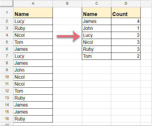
Ag ceapadh, tá liosta ainmneacha agat i gcolún A de bhileog Google, agus anois, ba mhaith leat a áireamh cé mhéad uair a thaispeántar gach ainm uathúil mar a thaispeántar ar an scáileán a thaispeántar. An rang teagaisc seo, labhróidh mé faoi roinnt foirmlí chun an post seo a réiteach ar bhileog Google.

Líon na dtarluithe i gcolún i mbileog Google le foirmle cúntóra

Líon na dtarluithe i gcolún i mbileog Google le foirmle


Líon na dtarluithe i gcolún i mbileog Google le foirmle cúntóra

Sa mhodh seo, is féidir leat na hainmneacha uathúla uile a bhaint as an gcolún ar dtús, agus ansin an tarlú a chomhaireamh bunaithe ar an luach uathúil.

1. Iontráil an fhoirmle seo le do thoil: = UNIQUE (A2: A16) isteach i gcill bhán inar mian leat na hainmneacha uathúla a bhaint, agus ansin brúigh Iontráil eochair, liostáladh na luachanna uathúla go léir mar a leanas a thaispeántar:

nótaí: San fhoirmle thuas, A2: A16 is iad na sonraí colúin is mian leat a chomhaireamh.

2. Agus ansin lean ar aghaidh leis an bhfoirmle seo a iontráil: = COUNTIF (A2: A16, C2) in aice leis an gcéad chill fhoirmle, brúigh Iontráil eochair chun an chéad toradh a fháil, agus ansin an láimhseáil líonta a tharraingt anuas go dtí na cealla ar mhaith leat tarlú na luachanna uathúla a chomhaireamh, féach an scáileán:

nótaí: San fhoirmle thuas, A2: A16 an bhfuil sonraí na gcolún ar mhaith leat ainmneacha uathúla a chomhaireamh uathu, agus C2 an chéad luach uathúil a bhain tú.


Líon na dtarluithe i gcolún i mbileog Google le foirmle

Is féidir leat an fhoirmle seo a leanas a chur i bhfeidhm freisin chun an toradh a fháil. Déan mar seo le do thoil:

Iontráil an fhoirmle seo le do thoil: = ArrayFormula (QUERY (A1: A16 & {"", ""}, "roghnaigh Col1, comhaireamh (Col2) áit a bhfuil Col1! = '' Grúpa de réir chomhaireamh lipéad Col1 (Col2) 'Líon'", 1)) isteach i gcill bhán inar mian leat an toradh a chur, ansin brúigh Iontráil eochair, agus an toradh ríofa curtha ar taispeáint ag an am céanna, féach an pictiúr:

nótaí: San fhoirmle thuas, A1: A16 an raon sonraí lena n-áirítear ceanntásc an cholúin a theastaíonn uait a chomhaireamh.


Líon na dtarluithe i gcolún i Microsoft Excel:

Kutools le haghaidh Excel'S Sraitheanna Comhcheangail Casta is féidir le fóntais cabhrú leat líon na dtarluithe i gcolún a chomhaireamh, agus féadann sé cabhrú leat luachanna comhfhreagracha cille a chomhcheangal nó a shuimiú bunaithe ar chealla céanna i gcolún eile.

Kutools le haghaidh Excel: le níos mó ná 300 breiseán áisiúil Excel, saor in aisce le triail gan aon teorannú i 30 lá. Íoslódáil agus triail saor in aisce Anois!

Uirlisí Táirgiúlachta Oifige is Fearr

🤖 Kutools AI Aide: anailís sonraí a réabhlóidiú bunaithe ar: Forghníomhú Chliste   |  Gin Cód  |  Cruthaigh Foirmlí Saincheaptha  |  Anailís a dhéanamh ar Sonraí agus Cairteacha a Ghin  |  Feidhmeanna Kutools a agairt...
Gnéithe Coitianta: Faigh, Aibhsigh nó Aithnigh Dúblaigh   |  Scrios Sraitheanna Bána   |  Comhcheangail Colúin nó Cealla gan Sonraí a Chailleadh   |   Babhta gan Foirmle ...
Cuardaigh Super: Ilchritéir VLookup    VLookup Illuachanna  |   VLookup Trasna Ilbhileoga   |   Amharc doiléir ....
Liosta anuas Casta: Go tapa Cruthaigh Liosta Anuas   |  Liosta anuas Cleithiúnach   |  Liosta Buail Isteach Ilroghnacha ....
Bainisteoir Colún: Cuir Líon Sonrach Colún leis  |  Colúin Bog  |  Scoránaigh Stádas Infheictheachta na gColún Ceilte  |  Déan comparáid idir Raonta & Colúin ...
Gnéithe Réadmhaoin: Fócas Eangaí   |  Amharc Dearaidh   |   Barra Mór na Foirmle    Leabhar Oibre & Bainisteoir Bileog   |  Leabharlann Acmhainní (Uaththéacs)   |  Piocálaí Dáta   |  Comhcheangail Bileoga Oibre   |  Criptigh/Díchriptigh Cealla    Seol Ríomhphost trí Liosta   |  Scagaire Super   |   Scagaire Speisialta (scagaire trom/iodálach/stailc tríd...) ...
Barr 15 Uirlisí12 Téacs uirlisí (Cuir Téacs, Bain Carachtair,...)   |   50 + Cairt cineálacha (Cairt Gantt,...)   |   40+ Praiticiúil Foirmlí (Ríomh aois bunaithe ar lá breithe,...)   |   19 Insertion uirlisí (Cuir isteach Cód QR, Ionsáigh Pictiúr ón gCosán,...)   |   12 Tiontú uirlisí (Uimhreacha le Focail, Comhshó Airgeadra,...)   |   7 Cumaisc & Scoilt uirlisí (Sraitheanna Comhcheangail Casta, Cealla Scoilt,...)   |   ... agus eile

Supercharge Do Scileanna Excel le Kutools le haghaidh Excel, agus Éifeachtúlacht Taithí Cosúil Ná Roimhe. Kutools le haghaidh Excel Tairiscintí Níos mó ná 300 Ardghnéithe chun Táirgiúlacht a Treisiú agus Sábháil Am.  Cliceáil anseo chun an ghné is mó a theastaíonn uait a fháil ...

Tuairisc


Tugann Tab Oifige comhéadan Tabbed chuig Office, agus Déan Do Obair i bhfad Níos Éasca

  • Cumasaigh eagarthóireacht agus léamh tabbed i Word, Excel, PowerPoint, Foilsitheoir, Rochtain, Visio agus Tionscadal.
  • Oscail agus cruthaigh cáipéisí iolracha i gcluaisíní nua den fhuinneog chéanna, seachas i bhfuinneoga nua.
  • Méadaíonn do tháirgiúlacht 50%, agus laghdaíonn sé na céadta cad a tharlaíonn nuair luch duit gach lá!
Comments (14)
No ratings yet. Be the first to rate!
This comment was minimized by the moderator on the site
可以限制规定内容出现的频次吗
This comment was minimized by the moderator on the site
Thanks!!! how do I count multiple columns?Ie column A, B,C,D all have names that needs to be counted
This comment was minimized by the moderator on the site
Thank you for this! Been trying to figure it out for hours!
This comment was minimized by the moderator on the site
Hi, I am trying to filter out some data from a sheet that is regularly updated. To simplify keeping track of the data I have a reporting section on the google sheet.The problem is that the data isn't organized in the most ideal way.

There are 2 columns that I want to use specific data from to create a filter, then with the leftover names I want to know how many unique names there are


Column 1 - Filter with A for one report field, B for the other report field (I will manually change this in the formula)

Column 2 - There are 9 Text entries possible. I want to only include 3 of them as a Filter

Column 3 - There are a couple of thousand entries(names), many are the same in multiple rows. With the data filtered using Column 1, and Column 2, I want to get a number for how many unique names are left after the data has been filtered.


I am not used to having this many things I am trying to filter the data from so any help would be hugely appreciated.


Have an excellent day
This comment was minimized by the moderator on the site
I have a google sheet with a lot of information but I am looking to filter it down into a report.

Column1 - Options are A, B (The is the first data to sort)
Column 2 - has 3 of the text string that I want my sum to include, but I want to leave out the others 5.
Column 3 - Names that I want to know how many unique names there are

What I am looking to figure out is the following

Option A, the sum to only include 3 text string that appears multiple times in a 2nd column, The total being how many unique names there are in Column 3

Hoping someone can help as this is a bit over my experience level
This comment was minimized by the moderator on the site
My count isn't grouping the names together.
i.e.
Column B says
Independence
Walnut St.
Parkway
Walnut St.
and instead of my " count " column saying Walnut St. 2 it says
Walnut St. 1
Walnut St. 1

How can I fix this ?
This comment was minimized by the moderator on the site
This is partly what I'm looking for.
Now my next issue is, how can I sort these so that I get them in desending order?
So it should be looking like this:
James 4
Nicol 3
Ruby 3
Lucy 2
Tom 2
John 1

Hope you can help with that as well
This comment was minimized by the moderator on the site
Hi,
If you want to sort the results in descending order, you just need to sort the data by the formula result column after getting the result.
Hope it can help you!
This comment was minimized by the moderator on the site
Whenever I try to sort, I get an error, is there a way I can fix that? I have the $A$1:$A$7, B1 as my formula - is there something in my formula I should edit?
This comment was minimized by the moderator on the site
VERY useful - thank you so much!
This comment was minimized by the moderator on the site
Thanks! Super useful!
This comment was minimized by the moderator on the site
When you drag the handle down to apply it to the rest of the values, it increments the search radius by 1. So if youre searching =COUNTIF(A1:A10,C1), when you drag the handle down, the second value will be =COUNTIF(A2:A11,C2).
This comment was minimized by the moderator on the site
This is SOOO helpful! This skips an entire step
This comment was minimized by the moderator on the site
You fix it this way
=COUNTIF($A$2:$A$11,C2)
There are no comments posted here yet
Please leave your comments in English
Posting as Guest
×
Rate this post:
0   Characters
Suggested Locations