Conas formáidiú coinníollach a dhéanamh bunaithe ar bhileog eile ar bhileog Google?
Más mian leat an fhormáidiú coinníollach a chur i bhfeidhm chun aird a tharraingt ar chealla atá bunaithe ar liosta sonraí ó bhileog eile mar an scáileán seo a leanas a thaispeántar ar bhileog Google, an bhfuil aon mhodhanna éasca agus maithe agat chun é a réiteach?
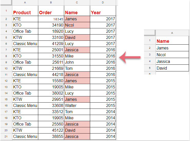
Formáidiú coinníollach chun aird a tharraingt ar chealla bunaithe ar liosta ó bhileog eile i Google Sheets

Déan na céimeanna seo a leanas le do thoil chun an post seo a chríochnú:
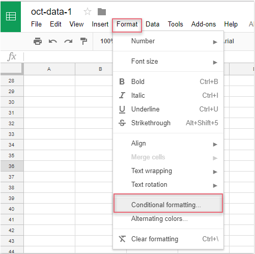
1. Cliceáil déanta > Formáidiú coinníollach, féach ar an scáileán:
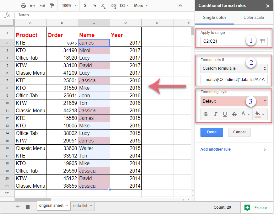
2. Sa an Rialacha formáide coinníollach pána, déan na hoibríochtaí seo a leanas le do thoil:
(1.) Cliceáil  cnaipe chun na sonraí colún a theastaíonn uait a aibhsiú a roghnú;
(2.) Sa Cealla formáid más rud é liosta anuas, roghnaigh le do thoil Is é an fhoirmle saincheaptha rogha, agus ansin cuir isteach an fhoirmle seo: = comhoiriúnú (C2, indíreach ("liosta sonraí! A2: A"), 0) isteach sa bhosca téacs;
(3.) Ansin roghnaigh formáidiú amháin as an Stíl formáidithe de réir mar is gá duit.
nótaí: San fhoirmle thuas: C2 Is í an chéad chill de na sonraí colúin ar mhaith leat aird a tharraingt orthu, agus an liosta sonraí! A2: A. is é ainm an bhileog agus raon na gcealla liosta ina bhfuil na critéir ar mhaith leat aird a tharraingt ar na cealla bunaithe orthu.
3. Agus aibhsíodh na cealla meaitseála uile atá bunaithe ar na cealla liosta ag an am céanna, ansin ba chóir duit cliceáil ar an Arna dhéanamh cnaipe chun an Rialacha formáide coinníollach pána mar is gá duit.
Uirlisí Táirgiúlachta Oifige is Fearr
Supercharge Do Scileanna Excel le Kutools le haghaidh Excel, agus Éifeachtúlacht Taithí Cosúil Ná Roimhe. Kutools le haghaidh Excel Tairiscintí Níos mó ná 300 Ardghnéithe chun Táirgiúlacht a Treisiú agus Sábháil Am. Cliceáil anseo chun an ghné is mó a theastaíonn uait a fháil ...
")
Tugann Tab Oifige comhéadan Tabbed chuig Office, agus Déan Do Obair i bhfad Níos Éasca
- Cumasaigh eagarthóireacht agus léamh tabbed i Word, Excel, PowerPoint, Foilsitheoir, Rochtain, Visio agus Tionscadal.
- Oscail agus cruthaigh cáipéisí iolracha i gcluaisíní nua den fhuinneog chéanna, seachas i bhfuinneoga nua.
- Méadaíonn do tháirgiúlacht 50%, agus laghdaíonn sé na céadta cad a tharlaíonn nuair luch duit gach lá!
")