
Conas vlookup a dhéanamh chun ilcholúin a chur ar ais ó thábla Excel?

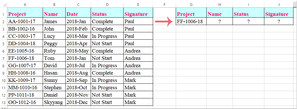
I mbileog oibre Excel, is féidir leat feidhm Vlookup a chur i bhfeidhm chun an luach meaitseála a thabhairt ar ais ó cholún amháin. Ach, uaireanta, b’fhéidir go mbeidh ort luachanna comhoiriúnaithe a bhaint as iliomad colúin mar a thaispeántar an pictiúr a leanas. Conas a d’fhéadfá na luachanna comhfhreagracha a fháil ag an am céanna ó ilcholúin tríd an bhfeidhm Vlookup a úsáid?

doc vlookup colúin iolracha 1

Vlookup chun luachanna meaitseála a thabhairt ar ais ó ilcholúin le foirmle eagar


Vlookup chun luachanna meaitseála a thabhairt ar ais ó ilcholúin le foirmle eagar

Anseo, tabharfaidh mé isteach feidhm Vlookup chun luachanna comhoiriúnaithe a thabhairt ar ais ó iliomad colúin, déan mar seo le do thoil:

1. Roghnaigh na cealla inar mian leat na luachanna meaitseála a chur ó ilcholúin, féach an scáileán:

doc vlookup colúin iolracha 2

2. Ansin cuir isteach an fhoirmle seo: =VLOOKUP(G2,A1:E13,{2,4,5},FALSE) isteach sa bharra foirmle, agus ansin brúigh Ctrl + Shift + Iontráil baineadh eochracha le chéile, agus baineadh na luachanna meaitseála ó cholúin iolracha ag an am céanna, féach an scáileán:

doc vlookup colúin iolracha 3

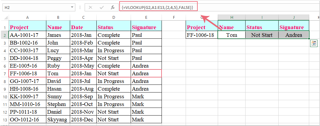
nótaí: San fhoirmle thuas, G2 an bhfuil na critéir ar mhaith leat luachanna a thabhairt ar ais bunaithe orthu, A1: E13 an raon tábla ar mhaith leat amharc air, an uimhir 2, 4, 5 is iad na huimhreacha colún ar mhaith leat luachanna a thabhairt ar ais uathu.

Uirlisí Táirgiúlachta Oifige is Fearr

🤖 Kutools AI Aide: anailís sonraí a réabhlóidiú bunaithe ar: Forghníomhú Chliste   |  Gin Cód  |  Cruthaigh Foirmlí Saincheaptha  |  Anailís a dhéanamh ar Sonraí agus Cairteacha a Ghin  |  Feidhmeanna Kutools a agairt...
Gnéithe Coitianta: Faigh, Aibhsigh nó Aithnigh Dúblaigh   |  Scrios Sraitheanna Bána   |  Comhcheangail Colúin nó Cealla gan Sonraí a Chailleadh   |   Babhta gan Foirmle ...
Cuardaigh Super: Ilchritéir VLookup    VLookup Illuachanna  |   VLookup Trasna Ilbhileoga   |   Amharc doiléir ....
Liosta anuas Casta: Go tapa Cruthaigh Liosta Anuas   |  Liosta anuas Cleithiúnach   |  Liosta Buail Isteach Ilroghnacha ....
Bainisteoir Colún: Cuir Líon Sonrach Colún leis  |  Colúin Bog  |  Scoránaigh Stádas Infheictheachta na gColún Ceilte  |  Déan comparáid idir Raonta & Colúin ...
Gnéithe Réadmhaoin: Fócas Eangaí   |  Amharc Dearaidh   |   Barra Mór na Foirmle    Leabhar Oibre & Bainisteoir Bileog   |  Leabharlann Acmhainní (Uaththéacs)   |  Piocálaí Dáta   |  Comhcheangail Bileoga Oibre   |  Criptigh/Díchriptigh Cealla    Seol Ríomhphost trí Liosta   |  Scagaire Super   |   Scagaire Speisialta (scagaire trom/iodálach/stailc tríd...) ...
Barr 15 Uirlisí12 Téacs uirlisí (Cuir Téacs, Bain Carachtair,...)   |   50 + Cairt cineálacha (Cairt Gantt,...)   |   40+ Praiticiúil Foirmlí (Ríomh aois bunaithe ar lá breithe,...)   |   19 Insertion uirlisí (Cuir isteach Cód QR, Ionsáigh Pictiúr ón gCosán,...)   |   12 Tiontú uirlisí (Uimhreacha le Focail, Comhshó Airgeadra,...)   |   7 Cumaisc & Scoilt uirlisí (Sraitheanna Comhcheangail Casta, Cealla Scoilt,...)   |   ... agus eile

Supercharge Do Scileanna Excel le Kutools le haghaidh Excel, agus Éifeachtúlacht Taithí Cosúil Ná Roimhe. Kutools le haghaidh Excel Tairiscintí Níos mó ná 300 Ardghnéithe chun Táirgiúlacht a Treisiú agus Sábháil Am.  Cliceáil anseo chun an ghné is mó a theastaíonn uait a fháil ...

Tuairisc


Tugann Tab Oifige comhéadan Tabbed chuig Office, agus Déan Do Obair i bhfad Níos Éasca

  • Cumasaigh eagarthóireacht agus léamh tabbed i Word, Excel, PowerPoint, Foilsitheoir, Rochtain, Visio agus Tionscadal.
  • Oscail agus cruthaigh cáipéisí iolracha i gcluaisíní nua den fhuinneog chéanna, seachas i bhfuinneoga nua.
  • Méadaíonn do tháirgiúlacht 50%, agus laghdaíonn sé na céadta cad a tharlaíonn nuair luch duit gach lá!
Comments (15)
No ratings yet. Be the first to rate!
This comment was minimized by the moderator on the site
how can i search for multiple lookup value?for eg: these two arrays shows diff freq coumn,gain,veritcal BW,tolerance etc.I want to get an average values gain and 3db BW..how can i enter the formula
y1    1800    7.5dBi +/- 2.9    22.1° +/- 6.8        7.5
y1    1900    7.6dBi +/- 3.0    18.9° +/- 3.6        7.6
y1    2100    6.7dBi +/- 2.6    17.7° +/- 3.6        6.7
y1    AWS    7.2dBi +/- 2.8    20.4° +/- 9.4        7.2
y1    2300    8.3dBi +/- 3.6    15.8° +/- 1.6        8.3
y1    2600    7.9dBi +/- 2.4    17.1° +/- 1.7        7.9
y2    1800    6.9dBi +/- 1.4    27.1° +/- 10.8        6.9
y2    1900    6.9dBi +/- 1.5    23.0° +/- 12.5        6.9
y2    2100    7.6dBi +/- 2.3    21.7° +/- 19.6        7.6
y2    AWS    8.0dBi +/- 2.5    23.3° +/- 13.8        8
y2    2300    7.7dBi +/- 1.6    15.9° +/- 5.9        7.7
y2    2600    6.5dBi +/- 2.3    14.5° +/- 3.9        6.5
This comment was minimized by the moderator on the site
I have many rows with same value but need to get multiple value after look up, I need to get two different EO ref , how can U##TRX EO
HXPRE-MQ1371 AB0024822
This comment was minimized by the moderator on the site
Thank you!! The { } of the columns is what I was missing. Appreciate this page!
This comment was minimized by the moderator on the site
Thanks! Super helpful, when other online options weren't
This comment was minimized by the moderator on the site
What if you need to have multiple rows as well? Ex. find all the FF-1006-18 rows while still only bringing back column B, D, and E.
This comment was minimized by the moderator on the site
Hello, Shelly,
Maybe there is not a direct formula for helping you, but, you can apply the below array fromula to get all matching values from the entire row, and then delete or hide the unwanted column as you need.
=INDEX($A$2:$E$10, SMALL(IF($G$2=$A$2:$A$10, ROW($A$2:$A$10)-MIN(ROW($A$2:$A$10))+1, ""), ROW(B1)),COLUMN(B1))
Then press Ctrl + Shift + Enter keys to get the first cell and then drag the fill handle to right and then drga down to get all corresponding values.

Please try, hope it can help you!
This comment was minimized by the moderator on the site
Thanks! This was really Helpful!
This comment was minimized by the moderator on the site
This method does not work. Even if it did, it is not the proper method.
Example of correct method is:
VLOOKUP($A2:$A1093, '[Workbook1.xlsx]Sheet2'!$A$2:$D$111,COLUMN(G2),FALSE)

Make sure you add $ before the column letter of your lookup reference to make sure it remains static, once done, using the filler button on the selected target cell, drag right to the corresponding number of columns.
This comment was minimized by the moderator on the site
This comment is exactly what I needed
This comment was minimized by the moderator on the site
How can I do this using 2 different spread sheets?
This comment was minimized by the moderator on the site
Hello, Lana,
The above formula in this article also can help you to get the results in another worksheet, you just need to change the cell reference as follows:
=VLOOKUP(A1,Sheet1!A1:E13,{2,4,5},FALSE)
Please remember to press Ctrl + Shift + Enter keys together to get the correct results.
This comment was minimized by the moderator on the site
NOT GETTING MULTIPLE COLUMN I'M GETTING ONLY ONE COLUMN VALUE
This comment was minimized by the moderator on the site
Hi, HARI,
To apply this formula, first, you should select the multiple cells where you want to output the results, and then copy the formula into the formula bar, then press Ctrl + Shift + Enter keys together to get the results.
Please try, hope it can help you!
This comment was minimized by the moderator on the site
This is great. How do I carry this formula down if I have 10,000 rows? I've tried a few ways but of course it's changing the formula on me.
This comment was minimized by the moderator on the site
Hi, Scully,
To apply this formula to multiple rows, you just need to change the relative cell reference to absolute reference, as this: =VLOOKUP(A1,Sheet1!$A$1:$E$13,{2,4,5},FALSE).
Please try this, hope it can help you!
There are no comments posted here yet
Please leave your comments in English
Posting as Guest
×
Rate this post:
0   Characters
Suggested Locations