
Conas luachanna meaitseála iolracha a thabhairt ar ais bunaithe ar chritéar amháin nó níos mó in Excel?

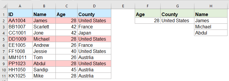
De ghnáth, is furasta don chuid is mó dínn luach sonrach a lorg agus an earra meaitseála a chur ar ais tríd an bhfeidhm VLOOKUP a úsáid. Ach, an ndearna tú iarracht riamh luachanna meaitseála iolracha a thabhairt ar ais bunaithe ar chritéar amháin nó níos mó mar a leanas an pictiúr a thaispeántar? San Airteagal seo, tabharfaidh mé isteach roinnt foirmlí chun an tasc casta seo a réiteach in Excel.

Cuir luachanna meaitseála iolracha ar ais bunaithe ar chritéar amháin nó níos mó le foirmlí eagar


Cuir luachanna meaitseála iolracha ar ais bunaithe ar chritéar amháin nó níos mó le foirmlí eagar

Mar shampla, ba mhaith liom gach ainm a bhfuil 28 bliana d’aois agus a thagann ó Stáit Aontaithe Mheiriceá a bhaint, cuir an fhoirmle seo a leanas i bhfeidhm:

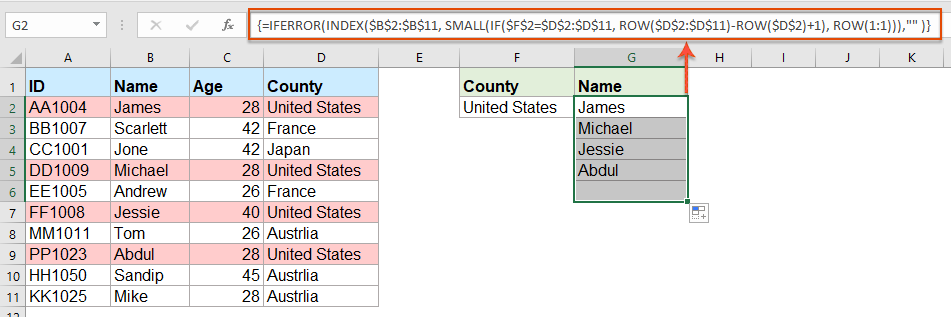
1. Cóipeáil nó cuir isteach an fhoirmle thíos i gcill bhán inar mian leat an toradh a aimsiú:

=INDEX($B$2:$B$11, SMALL(IF(COUNTIF($F$2, $C$2:$C$11)*COUNTIF($G$2, $D$2:$D$11), ROW($A$2:$D$11)-MIN(ROW($A$2:$D$11))+1), ROW(A1)), COLUMN(A1))

nótaí: San fhoirmle thuas, B2: B11 an colún é a gcuirtear an luach meaitseála ar ais uaidh; F2, C2: C11 arb iad an chéad choinníoll agus na sonraí colúin ina bhfuil an chéad choinníoll; G2, D2: D11 an dara coinníoll agus na sonraí colúin ina bhfuil an coinníoll seo, athraigh iad de réir do riachtanas.

2. Ansin, brúigh Ctrl + Shift + Iontráil eochracha chun an chéad toradh meaitseála a fháil, agus ansin an chéad chill fhoirmle a roghnú agus tarraing an láimhseáil líonta síos go dtí na cealla go dtí go dtaispeántar luach earráide, anois, tugtar na luachanna meaitseála uile ar ais mar atá thíos an scáileán a thaispeántar:

Leideanna: Mura gá duit ach na luachanna meaitseála uile a thabhairt ar ais bunaithe ar choinníoll amháin, cuir an fhoirmle eagar thíos i bhfeidhm:

=IFERROR(INDEX($B$2:$B$11, SMALL(IF($F$2=$D$2:$D$11, ROW($D$2:$D$11)-ROW($D$2)+1), ROW(1:1))),"" )


Earraí níos coibhneasta:

  • Luachanna Il-Amharc a Fhilleadh i gCill Scartha le Coma amháin
  • In Excel, is féidir linn feidhm VLOOKUP a chur i bhfeidhm chun an chéad luach comhoiriúnaithe a thabhairt ar ais ó chealla tábla, ach, uaireanta, caithfimid na luachanna meaitseála go léir a bhaint agus ansin iad a dheighilt le teorantóir ar leith, mar shampla camóg, Fleasc, srl. cill mar a thaispeántar an pictiúr a leanas. Conas a d’fhéadfaimis luachanna ilbhreathnaithe a fháil agus a thabhairt ar ais i gcill scartha camóg in Excel?
  • Luachanna Meaitseála Il Vlookup Agus Fill ar ais I mBileog Google Ag an am céanna
  • Is féidir leis an ngnáthfheidhm Vlookup i mbileog Google cabhrú leat an chéad luach meaitseála a fháil agus a chur ar ais bunaithe ar shonraí ar leith. Ach, uaireanta, b’fhéidir go mbeidh ort amharc agus filleadh ar na luachanna meaitseála go léir mar a leanas an pictiúr a thaispeántar. An bhfuil aon bhealaí maithe éasca agat chun an tasc seo a réiteach i mbileog Google?
  • Vlookup Agus Cuir Luachanna Il ar ais ón Liosta Buail Isteach
  • In Excel, conas a d’fhéadfá luachanna iolracha comhfhreagracha a bhreathnú agus a chur ar ais ó liosta anuas, rud a chiallaíonn nuair a roghnaíonn tú mír amháin ón liosta anuas, taispeántar a luachanna coibhneasta uile ag an am céanna mar a thaispeántar an pictiúr a leanas. An t-alt seo, tabharfaidh mé an réiteach isteach céim ar chéim.
  • Luachanna iomadúla a bhreathnú agus a thabhairt ar ais go hingearach in Excel
  • De ghnáth, is féidir leat feidhm Vlookup a úsáid chun an chéad luach comhfhreagrach a fháil, ach, uaireanta, ba mhaith leat gach taifead meaitseála a thabhairt ar ais bunaithe ar chritéar ar leith. An t-alt seo, labhróidh mé faoi conas na luachanna meaitseála go léir a bhreathnú agus a chur ar ais go hingearach, go cothrománach nó in aon chill amháin.
  • Vatchup Agus Sonraí Meaitseála a Fhilleadh Idir Dhá Luachan in Excel
  • In Excel, is féidir linn gnáthfheidhm Vlookup a chur i bhfeidhm chun an luach comhfhreagrach a fháil bunaithe ar shonraí ar leith. Ach, uaireanta, ba mhaith linn an luach meaitseála idir dhá luach a bhreathnú agus a chur ar ais mar a thaispeántar an pictiúr a leanas, conas a d’fhéadfá déileáil leis an tasc seo in Excel?


  • Barra Foirmle Super (cuir línte iolracha téacs agus foirmle in eagar go héasca); Leagan Amach Léitheoireachta (líon mór cealla a léamh agus a chur in eagar go héasca); Greamaigh go dtí an Raon Scagtha...
  • Cumaisc Cealla / Sraitheanna / Colúin agus Sonraí a Choinneáil; Ábhar Cealla Scoilt; Comhcheangail Sraitheanna Dúblacha agus Suim / Meán... Cill Dúblach a Chosc; Déan comparáid idir Ranganna...
  • Roghnaigh Dúblach nó Uathúil Sraitheanna; Roghnaigh Blank Rows (tá na cealla uile folamh); Aimsigh Super agus Fuzzy Aimsigh i go leor Leabhar Oibre; Roghnaigh go randamach ...
  • Cóip Díreach Cealla Il gan tagairt fhoirmle a athrú; Tagairtí Cruthaigh Auto chuig Bileoga Il; Cuir Urchair isteach, Boscaí Seiceála agus go leor eile ...
  • Foirmlí is Fearr agus Cuir isteach go tapa, Ranganna, Cairteacha agus Pictiúir; Cealla a Chriptiú le pasfhocal; Cruthaigh Liosta Ríomhphoist agus seol ríomhphoist ...
  • Sliocht Téacs, Cuir Téacs leis, Bain de réir Poist, Bain Spás; Subtotals Paging a chruthú agus a phriontáil; Tiontaigh Idir Ábhar Cealla agus Tráchtanna...
  • Scagaire Super (scéimeanna scagaire a shábháil agus a chur i bhfeidhm ar bhileoga eile); Ard-Sórtáil de réir míosa / seachtaine / lae, minicíocht agus níos mó; Scagaire Speisialta le cló trom, iodálach ...
  • Comhcheangail Leabhair Oibre agus Bileoga Oibre; Cumaisc Táblaí bunaithe ar eochaircholúin; Roinn Sonraí i Ilbhileoga; Baisc Tiontaigh xls, xlsx agus PDF...
  • Grúpáil Tábla Pivot de réir uimhir na seachtaine, lá na seachtaine agus níos mó ... Taispeáin Cealla Díghlasáilte, Faoi Ghlas de réir dathanna éagsúla; Aibhsigh Cealla a bhfuil Foirmle / Ainm orthu...
cluaisín kte 201905
  • Cumasaigh eagarthóireacht agus léamh tabbed i Word, Excel, PowerPoint, Foilsitheoir, Rochtain, Visio agus Tionscadal.
  • Oscail agus cruthaigh cáipéisí iolracha i gcluaisíní nua den fhuinneog chéanna, seachas i bhfuinneoga nua.
  • Méadaíonn do tháirgiúlacht 50%, agus laghdaíonn sé na céadta cad a tharlaíonn nuair luch duit gach lá!
bun officetab


Comments (25)
No ratings yet. Be the first to rate!
This comment was minimized by the moderator on the site
Hi, if there are duplicate values (e.g. two adams), how do i make sure that it only returns 1 adam and not 2?
This comment was minimized by the moderator on the site
Hello, Bobby,
To extract only unique matching values, you should apply the below formula:
After pasting the formula, please press Ctrl + Shift + Enter keys together to get the correct result.
=IFERROR(INDEX($B$2:$B$5, MATCH(0, COUNTIF(H1:$H$1, $B$2:$B$5)+IF($D$2:$D$5<>$G$2, 1, 0)+IF($C$2:$C$5<>$F$2, 1, 0), 0)), "")

Please have a try, hope it can help you!
This comment was minimized by the moderator on the site
Hi,

Thanks for posting these examples.
I'm trying to implement this in my own sheet, but don't get it to work (maybe because I'm using an europe version of excel)?

I want to get the dates of the days that I had my shifts or that I have worked 'some' (>0) hours for a client.

So in I3 is the name and in J3 the month. K3 and L3 are the shifts (1 is worked) and hours (don't know how to set this, should be more than zero)

My expected results are in:
Shifts: I7 and I8
hours: J7

So I worked more than 0 hours for 'person 2' in oktober on 3-10-2022
had shifts for person 2 on '10-10-2022' and 28-10-2022

When I add '=INDEX($B$2:$B$11, SMALL(IF(COUNTIF($F$2, $C$2:$C$11)*COUNTIF($G$2, $D$2:$D$11), ROW($A$2:$D$11)-MIN(ROW($A$2:$D$11))+1), ROW(A1)), COLUMN(A1))' in my excel sheet, it doesn't allow the comma between the different parts of the formula.
So I need to change them to ';'.
But when I try it it always says: '#NAME?'

So can someone help me with this?

Kind regards,

Bas
[img]https://drive.google.com/file/d/1iIPQKuj_PNhqWyWlwJ4IQTqGNEd6B9Hw/view?usp=share_link[/img]
This comment was minimized by the moderator on the site
Hi,

First, thank you for sharing!

Can you please provide a solution to the case below:

I have 3 columns (A: Containing reference information, B: Containing information to be searched, C: Search result)

Image url is provided below

https://ibb.co/VHCd09K

Column A-------------------------Column B------------Column C
File Name-------------------------Name----------------File Name, Document Name, Element Name, Name
Changed Element-----------------Element--------------Changed Element, Element Name, Element ID
Column Location
Document Name
Element Name
Name
Category
Warranty
Slope
Element ID

What I need is to search in column A for any partial match with cell B2 (Name) or B3 (Element) and get the result in one cell,

Thank you, Behzad
This comment was minimized by the moderator on the site
Hello, Behzad
Maybe the below User Defined Function can help you.
Public Function ConcatPartLookUp(rngInput As Range, rngSource As Range, Optional strDelimiter As String, Optional blCaseSensitive)
Dim rng As Range
If strDelimiter = "" Then strDelimiter = ","
If IsMissing(blCaseSensitive) Then
    blCaseSensitive = False
Else
    blCaseSensitive = True
End If
For Each rng In rngSource
    If blCaseSensitive Then
        If InStr(1, rng.Value, rngInput.Value, vbBinaryCompare) > 0 Then ConcatPartLookUp = ConcatPartLookUp & strDelimiter & rng.Value
    Else
        If InStr(1, rng.Value, rngInput.Value, vbTextCompare) > 0 Then ConcatPartLookUp = ConcatPartLookUp & strDelimiter & rng.Value
    End If
Next
If Len(ConcatPartLookUp) > 0 Then ConcatPartLookUp = Mid(ConcatPartLookUp, 2, Len(ConcatPartLookUp))
End Function


After copying and pasting this code, and then use this formula:=ConcatPartLookUp(B2,$A$2:$A$8) to get the result you need.
Please have a try, hope it can help you!
This comment was minimized by the moderator on the site
Heyi, thank you for the formula. It worked for "fixed" values / text as criterias. However, one of the criterias i'm trying to use is a condition (values <>0 ), but does not work the described formula. Do you guys know what should i change to adapt the formula so I can have a condition as one of the criterias, please?

Best,

João
This comment was minimized by the moderator on the site
Hello, Marcus
To solve your problem, please view this article:
https://www.extendoffice.com/documents/excel/6393-excel-vlookup-function.html#b3-2
There are some detailed explanations of this task. You just need to change the criteira to your own.
Thank you!
This comment was minimized by the moderator on the site
Hi,

if in cell H1 i write "Name" and wanted to link that with the formula, how would that work?
Then I could write "ID" in cell H1 and would automatically get as a result: AA1004; DD1009; PP1023 (for the first formula)

Thank you in advance!
This comment was minimized by the moderator on the site
Hello, Marie
Sorry, i can't get the point of your first problem, could you explain your problem more clearly and detailedly? Or you can insert a screenshot here to describe your problem.
As for the second question, you just need to change the cell reference as this:
=INDEX($A$2:$A$11, SMALL(IF(COUNTIF($F$2, $C$2:$C$11)*COUNTIF($G$2, $D$2:$D$11), ROW($A$2:$D$11)-MIN(ROW($A$2:$D$11))+1), ROW(A1)), COLUMN(A1))

Remeber to press Ctrl + Shift + Enter keys together.
Please try, hope it can help you!
This comment was minimized by the moderator on the site
Hello,
what would be needed to expand the first formula in the following case:
Some IDs are Blank (e.g. cell A5 is blank) and I would like an additional condition outputting lines only when the IDs are not blank. (So the output should then be James and Abdul.
Thanks!
This comment was minimized by the moderator on the site
Hello, Jo,
To solve your problem, please apply the below formula:
=INDEX($B$2:$B$11, SMALL(IF(COUNTIF($F$2, $C$2:$C$11)*COUNTIF($G$2, $D$2:$D$11)*($A$2:$A$11<>0), ROW($A$2:$D$11)-MIN(ROW($A$2:$D$11))+1), ROW(A1)), COLUMN(A1))

Please have a ry, hope it can help you!
This comment was minimized by the moderator on the site
hello,
ive tried using the formula and it either generates a value of 0 or the image attached
This comment was minimized by the moderator on the site
Hello, Milku
Your screenshot showed WPS software of MAC version, so I am not sure whether our formula is available.
I uploaded an Excel file to here, you can try to see if it can calculate correctly in you environment.
Thank you!
This comment was minimized by the moderator on the site
When I use the second formula and drag down, nothing appears. The formula result (fx) says it should be returning something but it is blank. How do I correct this?
This comment was minimized by the moderator on the site
Hello Alysia,

Glad to help. I tried the second formula in the article and drag the formula down, the rest of results were returned. I think there may be two reasons for your problem. First, maybe you forget to press Ctrl + Shift + Enter keys to enter the formula. Second, the matching result is only one, so no other results are not returned. Please have a check.

Sincerely,
Mandy
This comment was minimized by the moderator on the site
Hi,

I was wondering if it at all possible to enter a 2nd criteria but from the same range as the 1st criteria,

For example with the used example above i would like to search for the names of people from both America and France So cell F3 would have France, Scarlett & Andrew would also populate in the list in Column G

Thank you for assistance in advance.
This comment was minimized by the moderator on the site
Hello Nick,

Glad to help. If you want to get the names of people from both America and France, I advise you to use our formula twice to get the result. Please see the screenshot, In F2 and G2 are values "United States" and "France". Apply formula =IFERROR(INDEX($B$2:$B$11, SMALL(IF($F$2=$D$2:$D$11, ROW($D$2:$D$11)-ROW($D$2)+1), ROW(1:1))),"" ) to get the results for America. And apply formula =IFERROR(INDEX($B$2:$B$11, SMALL(IF($G$2=$D$2:$D$11, ROW($D$2:$D$11)-ROW($D$2)+1), ROW(1:1))),"" ) to get the results for France. It's simple. Please have a try.

Sincerely,
Mandy
This comment was minimized by the moderator on the site
In the first example, what change to the formula would be needed to return everyone who was less than 28 years old?
There are no comments posted here yet
Load More
Please leave your comments in English
Posting as Guest
×
Rate this post:
0   Characters
Suggested Locations