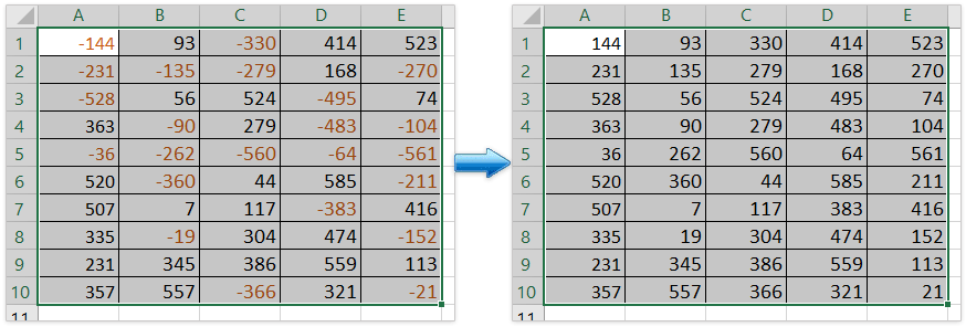
Is féidir leat na huimhreacha diúltacha a athrú go huimhreacha dearfacha leis na céimeanna seo a leanas:

1. Iontráil uimhir -1 i gcill bhán, ansin roghnaigh an cill seo, agus brúigh Ctrl + C eochracha chun é a chóipeáil.

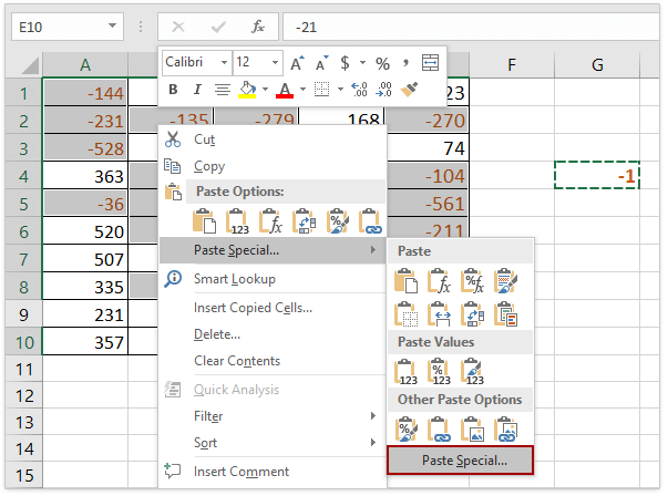
2. Roghnaigh gach uimhir dhiúltach sa raon, cliceáil ar dheis, agus roghnaigh Greamaigh Speisialta ... ón roghchlár comhthéacs. Féach an pictiúr:

Nótaí:
(1) Gabháltas Ctrl eochair, is féidir leat gach uimhir dhiúltach a roghnú ach iad a chliceáil ceann ar cheann;
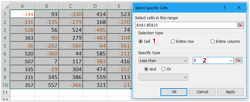
(2) Má tá Kutools for Excel suiteáilte agat, is féidir leat a chuid a chur i bhfeidhm Roghnaigh Cealla Speisialta gné chun gach uimhir dhiúltach a roghnú go tapa. Bíodh Triail In Aisce agat!

3. Agus a Greamaigh speisialta taispeánfar bosca dialóige, roghnaigh Gach rogha ó Greamaigh, Roghnaigh Méadaigh rogha ó Oibríocht, Cliceáil OK. Féach an pictiúr:

4. Athrófar na huimhreacha diúltacha uile a roghnófar ina huimhreacha dearfacha. Scrios an uimhir -1 de réir mar is gá duit. Féach an pictiúr:

Athraigh uimhreacha diúltacha go dearfach go dearfach sa raon sonraithe in Excel

Ag comparáid leis an gcomhartha diúltach a bhaint de chealla ceann ar cheann de láimh, Kutools for Excel's Athraigh Comhartha Luachanna Soláthraíonn gné bealach thar a bheith éasca chun gach uimhir dhiúltach a athrú go tapa go dearfach sa roghnú.

Mar ghairmí Excel, is féidir leat an cód VBA a rith freisin chun na huimhreacha diúltacha a athrú go huimhreacha dearfacha.

1. Brúigh eochracha Alt + F11 chun an fhuinneog Microsoft Visual Basic for Applications a oscailt.

2. Beidh fuinneog nua ar taispeáint. Cliceáil Ionsáigh > Modúil, ansin na cóid seo a leanas a ionchur sa mhodúl:

Sub Positive
Dim Cel As Range
For Each Cel In Selection
If IsNumeric(Cel.Value) Then
Cel.Value = Abs(Cel.Value)
End If
Next Cel
End Sub

3. Ansin cliceáil Rith cnaipe nó brúigh F5 eochair chun an feidhmchlár a rith, agus athrófar gach uimhir dhiúltach go huimhreacha dearfacha. Féach an pictiúr:

Níl an chuid is mó d’úsáideoirí Excel ag iarraidh cód VBA a úsáid, an bhfuil aon chleasanna gasta ann chun na huimhreacha diúltacha a athrú go dearfach? Kutools ar fheabhas in ann cabhrú leat go héasca agus go compordach chun é seo a bhaint amach.

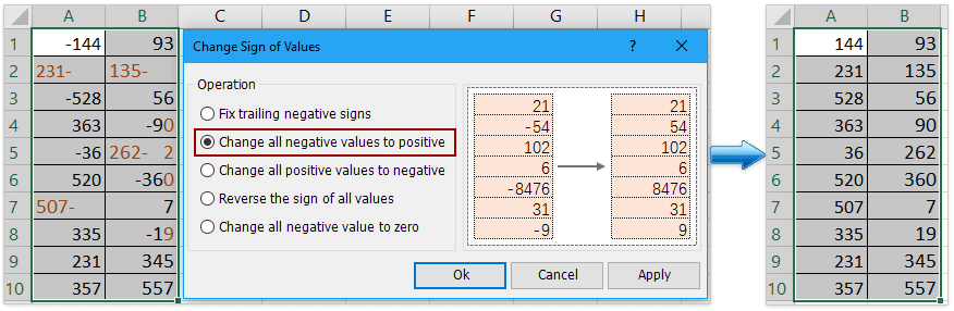
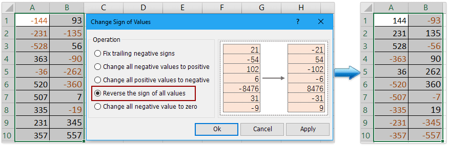
1. Roghnaigh raon lena n-áirítear na huimhreacha diúltacha a theastaíonn uait a athrú, agus cliceáil Kutools > Ábhar > Athraigh Comhartha Luachanna.

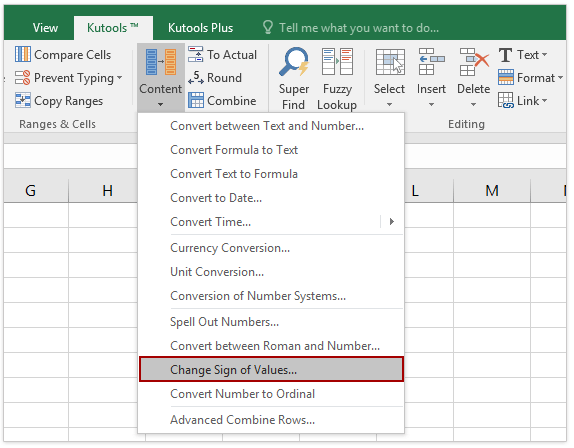
2. Seiceáil Athraigh gach luach diúltach go dearfach faoi Oibríocht, agus cliceáil Ok. Féach an pictiúr:

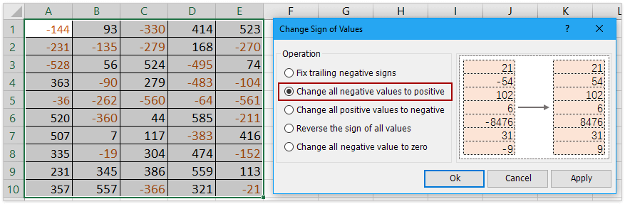
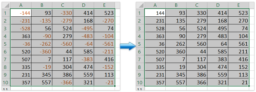
Anois feicfidh tú go n-athróidh na huimhreacha diúltacha go huimhreacha dearfacha mar a thaispeántar thíos:

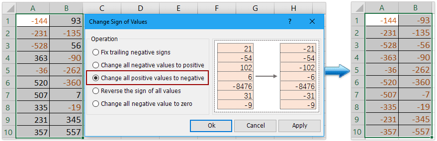
nótaí: Leis seo Athraigh comhartha Luachanna gné, is féidir leat comharthaí diúltacha rianaithe a shocrú freisin, gach uimhir dhearfach a athrú go diúltach, comhartha na luachanna uile a aisiompú agus gach luach diúltach a athrú go nialas. Bíodh Triail In Aisce agat!

(1) Athraigh go tapa na luachanna dearfacha go diúltach sa raon sonraithe:

(2) Comhartha na luachanna uile sa raon sonraithe a aisiompú go héasca:

(3) Gach luach diúltach a athrú go nialas sa raon sonraithe:

(4) Comharthaí diúltacha rianaithe a shocrú go héasca sa raon sonraithe:

Athraigh uimhreacha dearfacha go diúltach

Comharthaí droim ar ais luachanna i gcealla

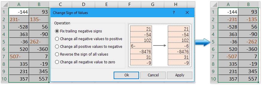
Deisigh comharthaí diúltacha trailing i gcealla

Athraigh uimhir dhiúltach go nialas