Conas dath cúlra nó cló a athrú bunaithe ar luach cille in Excel?
Nuair a dhéileálann tú le sonraí ollmhóra in Excel, b’fhéidir gur mhaith leat luach éigin a roghnú agus aird a tharraingt orthu le cúlra nó dath cló sonrach. Tá an t-alt seo ag caint ar conas an cúlra nó dath an chló a athrú bunaithe ar luachanna cille in Excel go tapa.
Modh 1: Athraigh dath cúlra nó cló bunaithe ar luach cille go dinimiciúil le Formáidiú Coinníollach
Modh 2: Athraigh dath cúlra nó cló bunaithe ar luach cille go statach leis an bhfeidhm Aimsigh
Modh 3: Athraigh dath cúlra nó cló bunaithe ar luach cille go statach le Kutools for Excel
Modh 1: Athraigh dath cúlra nó cló bunaithe ar luach cille go dinimiciúil le Formáidiú Coinníollach
An Formáidiú Coinníollach is féidir le gné cabhrú leat aird a tharraingt ar na luachanna is mó ná x, níos lú ná y, nó idir x agus y.
Má tá raon sonraí agat, agus anois go gcaithfidh tú na luachanna idir 80 agus 100 a dhathú, déan na céimeanna seo a leanas le do thoil:
1. Roghnaigh an raon cealla ar mhaith leat aird a tharraingt ar chealla áirithe, agus ansin cliceáil Baile > Formáidiú Coinníollach > Riail Nua, féach ar an scáileán:

2. Sa an Riail Nua Formáidithe bosca dialóige, roghnaigh an Formáid ach cealla ina bhfuil mír sa Roghnaigh Cineál Riail bosca, agus sa Formáid Amháin Cealla le alt, sonraigh na coinníollacha a theastaíonn uait:
- Sa chéad bhosca anuas, roghnaigh an Luach Cill;
- Sa dara bosca anuas, roghnaigh na critéir:idir;
- Sa tríú agus sa cheathrú bosca, iontráil na coinníollacha scagaire, mar shampla 80, 100.

3. Ansin, cliceáil déanta cnaipe, sa Cealla Formáid bosca dialóige, socraigh an cúlra nó an dath cló mar seo:
| Athraigh dath an chúlra de réir luach cille: | Athraigh dath an chló de réir luach cille |
| cliceáil Líon cluaisín, agus ansin roghnaigh dath cúlra amháin is mian leat | cliceáil Cló cluaisín, agus roghnaigh an dath cló atá uait. |
 |
 |
4. Tar éis dath an chúlra nó an chló a roghnú, cliceáil OK > OK chun na dialóga a dhúnadh, agus anois, athraítear na cealla ar leith a bhfuil luach idir 80 agus 100 acu go cinnte an cúlra nó an dath cló sa roghnú. Féach an pictiúr:
| Aibhsigh cealla ar leith a bhfuil dath cúlra orthu: | Aibhsigh cealla ar leith le dath cló: |
 |
 |
nótaí: An Formáidiú Coinníollach is gné dhinimiciúil é, athrófar dath na cille de réir mar a athraíonn na sonraí.
Modh 2: Athraigh dath cúlra nó cló bunaithe ar luach cille go statach leis an bhfeidhm Aimsigh
Uaireanta, ní mór duit dath líonta nó cló sonrach a chur i bhfeidhm bunaithe ar luach cille agus a dhéanamh nach n-athraíonn an dath líonta nó cló nuair a athraíonn luach na cille. Sa chás seo, is féidir leat an Aimsigh feidhm chun na luachanna sonracha cille go léir a fháil agus ansin an cúlra nó an dath cló a athrú de réir do riachtanas.
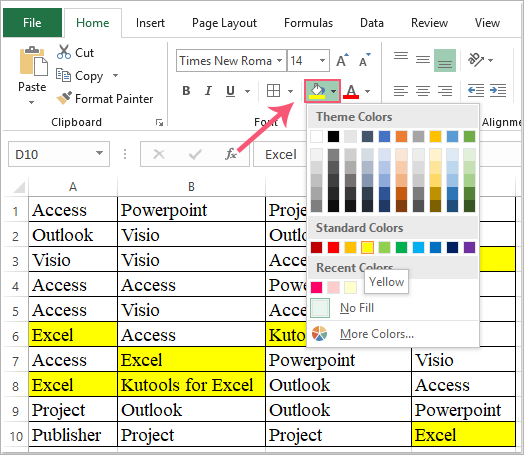
Mar shampla, ba mhaith leat an cúlra nó an dath cló a athrú má tá téacs “Excel” sa luach cille, déan mar seo é le do thoil:
1. Roghnaigh an raon sonraí a theastaíonn uait a úsáid, agus ansin cliceáil Baile > Faigh & Roghnaigh > Aimsigh, féach ar an scáileán:

2. Sa an Aimsigh agus Ionadaigh bosca dialóige, faoin Aimsigh cluaisín, cuir isteach an luach is mian leat a fháil isteach sa Aimsigh cad bosca téacs, féach an pictiúr:

3. Agus ansin, cliceáil Faigh Gach cnaipe, sa bhosca toradh aimsithe, cliceáil aon earra amháin, agus ansin brúigh Ctrl + A chun gach earra a aimsíodh a roghnú, féach an scáileán:

4. Faoi dheireadh, cliceáil Dún cnaipe chun an dialóg seo a dhúnadh. Anois, is féidir leat cúlra nó dath cló a líonadh do na luachanna roghnaithe seo, féach an scáileán:
| Cuir an dath cúlra i bhfeidhm ar na cealla roghnaithe: | Cuir dath an chló i bhfeidhm ar na cealla roghnaithe: |
 |
 |
Modh 3: Athraigh dath cúlra nó cló bunaithe ar luach cille go statach le Kutools for Excel
Kutools le haghaidh Excel'S Super Aimsigh Tacaíonn an ghné le go leor coinníollacha chun luachanna, teaghráin téacs, dátaí, foirmlí, cealla formáidithe agus mar sin de a fháil. Tar éis duit na cealla comhoiriúnaithe a aimsiú agus a roghnú, is féidir leat an cúlra nó an dath cló a athrú go dtí an rud atá uait.
Tar éis a shuiteáil Kutools le haghaidh Excel, déan mar seo le do thoil:
1. Roghnaigh an raon sonraí a theastaíonn uait a fháil, agus ansin cliceáil Kutools > Super Aimsigh, féach ar an scáileán:

2. Sa an Super Aimsigh pána, déan na hoibríochtaí seo a leanas le do thoil:
- (1.) Ar dtús, cliceáil an luachanna deilbhín rogha;
- (2.) Roghnaigh an scóip aimsithe ón Laistigh de titim anuas, sa chás seo, roghnóidh mé Roghnú;
- (3.) Ón cineál liosta anuas, roghnaigh na critéir is mian leat a úsáid;
- (4.) Ansin cliceáil Aimsigh cnaipe chun na torthaí comhfhreagracha uile a liostáil sa bhosca liosta;
- (5.) Faoi dheireadh, cliceáil Roghnaigh cnaipe chun na cealla a roghnú.

3. Agus ansin, roghnaíodh na cealla go léir a mheaitseálann na critéir ag an am céanna, féach an scáileán:

4. Agus anois, is féidir leat an dath cúlra nó an dath cló do na cealla roghnaithe a athrú de réir mar is gá duit.
Leideanna: Leis an Super Aimsigh feidhm, is féidir leat déileáil leis na hoibríochtaí seo a leanas go tapa agus go héasca:
Obair ghnóthach ar an deireadh seachtaine, Úsáid Kutools le haghaidh Excel,
tugann sé deireadh seachtaine suaimhneach, lúcháireach duit!
Ag an deireadh seachtaine, tá na páistí ag clamáil le dul amach ag imirt, ach tá an iomarca oibre thart timpeall ort chun am a bheith agat leis an teaghlach. An ghrian, an trá agus an fharraige go dtí seo? Kutools le haghaidh Excel Cabhraíonn a thabhairt duit réiteach puzzles Excel, sábháil am oibre.

- Faigh ardú céime agus níl tuarastal méadaithe i gcéin;
- Tá ardghnéithe ann, cásanna iarratais a réiteach, sábhálann roinnt gnéithe fiú 99% am oibre;
- Bí i do shaineolaí Excel i gceann 3 nóiméad, agus faigh aitheantas ó do chomhghleacaithe nó ó do chairde;
- Ní gá réitigh a chuardach ó Google a thuilleadh, slán a fhágáil le foirmlí pianmhara agus cóid VBA;
- Is féidir gach oibríocht arís agus arís eile a chur i gcrích gan ach cúpla cad a tharlaíonn, saor do lámha tuirseach;
- Níl ach $ 39 ach fiú níos mó ná rang teagaisc Excel $ 4000 na ndaoine eile;
- A bheith roghnaithe ag 110,000 mionlach agus 300+ cuideachta mór le rá;
- Triail saor in aisce 30 lá, agus airgead iomlán ar ais laistigh de 60 lá gan chúis ar bith;
- Athraigh an bealach ina n-oibríonn tú, agus ansin athraigh do stíl mhaireachtála!