
Conas luachanna a shuimiú idir dhá dháta in Excel?

Nuair a bhíonn dhá liosta i do bhileog oibre mar an scáileán ceart a thaispeántar, is é ceann liosta na ndátaí, is é an ceann eile liosta na luachanna. Agus ba mhaith leat na luachanna idir raon dhá dháta a achoimriú, mar shampla, na luachanna idir 3/4/2014 agus 5/10/2014 a achoimriú, conas is féidir leat iad a ríomh go tapa? Anois, tugaim isteach foirmle chun tú a achoimriú in Excel.


Luachanna suime idir dhá dháta leis an bhfoirmle in Excel

Ar ámharaí an tsaoil, tá foirmle ann ar féidir léi na luachanna idir raon dhá dháta in Excel a achoimriú.

Roghnaigh cill bhán agus clóscríobh isteach san fhoirmle thíos, agus brúigh Iontráil cnaipe. Agus anois gheobhaidh tú an toradh ríofa. Féach an pictiúr:

=SUMIFS(B2:B8,A2:A8,">="&E2,A2:A8,"<="&E3)

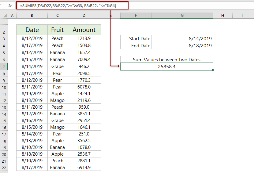
nótaí: San fhoirmle thuas,

  • D3: D22 an liosta luacha a thabharfaidh tú achoimre air
  • B3: B22 an bhfuil an liosta dáta a ndéanfaidh tú suim air bunaithe ar
  • G3 an cill le dáta tosaithe
  • G4 an cill le dáta deiridh
ribín nóta Tá an fhoirmle ró-chasta le cuimhneamh? Sábháil an fhoirmle mar iontráil Auto Text le haghaidh athúsáid agus gan ach cliceáil amháin sa todhchaí!
Léigh níos mó ...     Triail saor in aisce

Déan sonraí a shuimiú go héasca i ngach bliain fioscach, gach leathbhliain, nó gach seachtain in Excel

Tá an ghné Grúpáil Ama Speisialta PivotTable, arna sholáthar ag Kutools le haghaidh Excel, in ann colún cúntóra a chur leis chun an bhliain fhioscach, leathbhliain, uimhir seachtaine, nó lá na seachtaine a ríomh bunaithe ar an gcolún dáta sonraithe, agus ligean duit comhaireamh, suim a dhéanamh go héasca , nó meáncholúin bunaithe ar na torthaí ríofa i dTábla Pivot nua.


Kutools le haghaidh Excel - Supercharge Excel le níos mó ná 300 uirlisí riachtanacha. Bain sult as triail iomlán 30-lá SAOR IN AISCE gan aon chárta creidmheasa ag teastáil! Get sé anois


Luachanna suime idir dhá dháta leis an scagaire in Excel

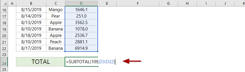
Más gá duit luachanna a shuimiú idir dhá dháta, agus go n-athraíonn an raon dáta go minic, is féidir leat scagaire a chur leis an raon áirithe, agus ansin an fheidhm SUBTOTAL a úsáid chun suim a dhéanamh idir an raon dáta sonraithe in Excel.

1. Roghnaigh cill bhán, iontráil thíos an fhoirmle, agus brúigh an Iontráil eochair.

= SUBTOTAL (109, D3: D22)

Nóta: San fhoirmle thuas, ciallaíonn 109 luachanna scagtha suime, léiríonn D3: D22 an liosta luacha a dhéanfaidh tú a achoimriú.

2. Roghnaigh teideal an raoin, agus cuir scagaire leis trí chliceáil Dáta > scagairí.

3. Cliceáil deilbhín an scagaire i gceanntásc an cholúin Dáta, agus roghnaigh Scagairí Dáta > Idir. Sa dialóg Saincheaptha AutoFilter, clóscríobh an dáta tosaigh agus an dáta deiridh de réir mar a theastaíonn uait, agus cliceáil ar an OK cnaipe. Athróidh an luach iomlán go huathoibríoch bunaithe ar luachanna scagtha.


Earraí gaolmhara:

Uirlisí Táirgiúlachta Oifige is Fearr

🤖 Kutools AI Aide: anailís sonraí a réabhlóidiú bunaithe ar: Forghníomhú Chliste   |  Gin Cód  |  Cruthaigh Foirmlí Saincheaptha  |  Anailís a dhéanamh ar Sonraí agus Cairteacha a Ghin  |  Feidhmeanna Kutools a agairt...
Gnéithe Coitianta: Faigh, Aibhsigh nó Aithnigh Dúblaigh   |  Scrios Sraitheanna Bána   |  Comhcheangail Colúin nó Cealla gan Sonraí a Chailleadh   |   Babhta gan Foirmle ...
Cuardaigh Super: Ilchritéir VLookup    VLookup Illuachanna  |   VLookup Trasna Ilbhileoga   |   Amharc doiléir ....
Liosta anuas Casta: Go tapa Cruthaigh Liosta Anuas   |  Liosta anuas Cleithiúnach   |  Liosta Buail Isteach Ilroghnacha ....
Bainisteoir Colún: Cuir Líon Sonrach Colún leis  |  Colúin Bog  |  Scoránaigh Stádas Infheictheachta na gColún Ceilte  |  Déan comparáid idir Raonta & Colúin ...
Gnéithe Réadmhaoin: Fócas Eangaí   |  Amharc Dearaidh   |   Barra Mór na Foirmle    Leabhar Oibre & Bainisteoir Bileog   |  Leabharlann Acmhainní (Uaththéacs)   |  Piocálaí Dáta   |  Comhcheangail Bileoga Oibre   |  Criptigh/Díchriptigh Cealla    Seol Ríomhphost trí Liosta   |  Scagaire Super   |   Scagaire Speisialta (scagaire trom/iodálach/stailc tríd...) ...
Barr 15 Uirlisí12 Téacs uirlisí (Cuir Téacs, Bain Carachtair,...)   |   50 + Cairt cineálacha (Cairt Gantt,...)   |   40+ Praiticiúil Foirmlí (Ríomh aois bunaithe ar lá breithe,...)   |   19 Insertion uirlisí (Cuir isteach Cód QR, Ionsáigh Pictiúr ón gCosán,...)   |   12 Tiontú uirlisí (Uimhreacha le Focail, Comhshó Airgeadra,...)   |   7 Cumaisc & Scoilt uirlisí (Sraitheanna Comhcheangail Casta, Cealla Scoilt,...)   |   ... agus eile

Supercharge Do Scileanna Excel le Kutools le haghaidh Excel, agus Éifeachtúlacht Taithí Cosúil Ná Roimhe. Kutools le haghaidh Excel Tairiscintí Níos mó ná 300 Ardghnéithe chun Táirgiúlacht a Treisiú agus Sábháil Am.  Cliceáil anseo chun an ghné is mó a theastaíonn uait a fháil ...

Tuairisc


Tugann Tab Oifige comhéadan Tabbed chuig Office, agus Déan Do Obair i bhfad Níos Éasca

  • Cumasaigh eagarthóireacht agus léamh tabbed i Word, Excel, PowerPoint, Foilsitheoir, Rochtain, Visio agus Tionscadal.
  • Oscail agus cruthaigh cáipéisí iolracha i gcluaisíní nua den fhuinneog chéanna, seachas i bhfuinneoga nua.
  • Méadaíonn do tháirgiúlacht 50%, agus laghdaíonn sé na céadta cad a tharlaíonn nuair luch duit gach lá!
Comments (48)
No ratings yet. Be the first to rate!
This comment was minimized by the moderator on the site
INVOICE DATE TOTAL
01-09-2021 19817
02-09-2021 44791
03-09-2021 26780
03-09-2021 58500
03-09-2021 2029

04-09-2021 79260
04-09-2021 2120
04-09-2021 9187
04-09-2021 5698
04-09-2021 1400
04-09-2021 1900
04-09-2021 7500
04-09-2021 830


i have above data in one sheet and i need date wise total value as below in another sheet,01-09-2021 19817
02-09-2021 44791
03-09-2021 87309
04-09-2021 107895

pls give formula details for itsanjay
This comment was minimized by the moderator on the site
Hi Jett,
You can use the SUMIFS function to sum by multiple criteria simultaneously.
=SUMIFS(sum_range, criteria_range1, criteria1, criteria_range2, criteria2,…, criteria_rangeN, criteriaN)
This comment was minimized by the moderator on the site
What if there are multiple columns to sum up like one for interest, one for penalty, and one for principal amount? and it still need to be between two dates
This comment was minimized by the moderator on the site
hi i have a question related to your topic,if the case is like thisDATE AMOUNT17 SEP 70.000 60.00018 SEP 30.00019 SEP 20.000 10.000IF i use sum if between date 17 sept to 19 sept the 60.000 & 10.000 can't be include in the total.what formulas should i use to include the 60.000 and 10.000 in the total?
This comment was minimized by the moderator on the site
Hi, i have a question related to sumifs:

want to calculate a sum between two dates e.g. start of date and end of date, but at times there are payments which were made in a new month but connected to the expense month, For example if a payment date is Oct 5th but the payment is for September and I would like to show this payment for the month of September, the formula should ignore the Oct 5th date and consider the payment in September. How do i do that
This comment was minimized by the moderator on the site
Help! I can only get this formula to work if I convert to a MM/DD/YYYY format but all of my data is DD/MM/YYYY. The cells are formatted correctly but the formula doesn't work unless I change from eg. 14/01/2020 to 01/14/2020.
This comment was minimized by the moderator on the site
Hi,

can you help me to calculate two working experiences in excel.

Ex: 12 Yeas 3 Months 5 Days - CDB Finance company

9 Years 4 Months 7 Days - Commercial Bank

These are two working experiences in two working places of one person. how to sum these two experiences as a total experience in excel. Please help me.
This comment was minimized by the moderator on the site
Hi Ayesha,
We can suppose the start is 1900/1/0, and add the two date periods to get the end date, and then get the difference between the start date and end date as attached image shown.
Two formulas used:
In Cell B7: =DATE(YEAR(0)+B4+B5,MONTH(0)+C4+C5,DAY(0)+D4+D5)
In Cell B9: =DATEDIF(B1,B7,"Y")&" Years, "&DATEDIF(B1,B7,"YM")&" Months, "&DATEDIF(B1,B7,"MD")&" Days"
This comment was minimized by the moderator on the site
Hi all,

What if one would like to make a date range non-mandatory?

Meaning, let's say that I have two cells with dates in them that are used as my beginning and end date threshold, but when those cells aren't populated, the sum for all dates is pulled from the data set.

My formula (below) has two match criteria with the date ranges at the back of the formula. What I'm trying to do is only filter the sum by the date range if a condition is met (ideally a cell that acts as select Yes or No on "Do you want to limit the sum to a specific date range?"

=SUMIFS(BURN_DATA!$S:$S,BURN_DATA!$R:$R,$A12,BURN_DATA!$H:$H,I$3,BURN_DATA!O:O,">="&I9,BURN_DATA!O:O,"<="&J9)


THANKS IN ADVANCE!
This comment was minimized by the moderator on the site
Aloha, I'm trying to figure out how to sum another column of units, when one column of dates is sequential. Example: I have rows with dates, Mar 1, Mar 2, mar3, then marc 6,7, then march 10.
I need to sum the corresponding units in of another column for mar 1-3, mar 6-7 and mar 10.
This comment was minimized by the moderator on the site
Hi David,
You can use methods introduced in this webpage to sum each period one by one.
Or you can add a helper column before the date column as attached image shown, and then apply the Subtotal feature.
This comment was minimized by the moderator on the site
I am trying to create a holiday calendar to calculate the following information:

Start Date:
End Date (if there is one, otherwise calculate on the entire holiday year_
No of Holidays
Holiday year runs from 01/04 to 31/03 with an entitlement of 20 days plus bank holidays

any help is much appreciated
There are no comments posted here yet
Load More
Please leave your comments in English
Posting as Guest
×
Rate this post:
0   Characters
Suggested Locations