Conas an chéad luach eile is mó in Excel a fheiceáil?
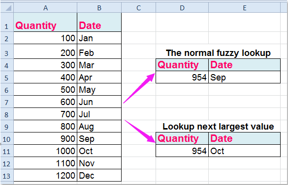
Have you ever noticed that when you apply the VLOOKUP function to extract the approximate matched value by using this formula: =VLOOKUP(D2,A2:B8,2,TRUE), you will get the value less than the lookup value. However, in certain situations, you might need to find the next largest record. Look at the following example, I want to look up the corresponding date of quantity 954, now, I want it to return the date which has the higher value than 954 in the VLOOKUP, so Oct rather than Sep. In this article, I can talk about how to lookup next largest value and return its relative data in Excel.
Vlookup the next largest value and return its corresponding data with formulas
 Vlookup the next largest value and return its corresponding data with formulas
To deal with this task, the following formulas may help you, please do as follows:
1. Please enter this array formula: =INDEX(B2:B13,MATCH(TRUE,A2:A13>D5,0)) isteach i gcill bhán inar mian leat an toradh a chur, féach an pictiúr:
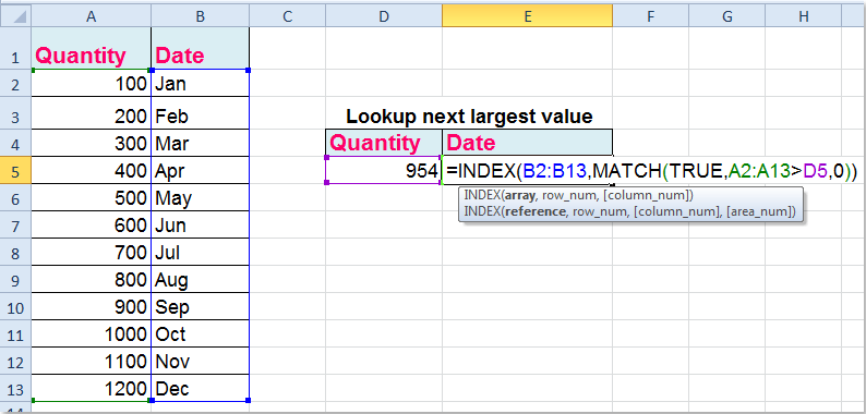
2. Ansin brúigh Ctrl + Shift + Iontráil keys together to get the correct result you need as follows:

Nótaí:
1. Excepting the above array formula, here also is another normal formula: =INDEX(B2:B13,MATCH(D5,A2:A13)+(LOOKUP(D5,A2:A13)<>D5)), after typing this formula and just press Iontráil key to find the next largest value and return its corresponding value.
2. Sna foirmlí thuas, B2: B13 is the data range that you want to extract the matched value, A2: A13 is the data range including the criterion that you want to lookup from , and D5 indicates the criteria you want to get its relative value of adjacent column, you can change them to your need.
Earraí gaolmhara:
Conas amharc i dtábla déthoiseach in Excel?
Conas amharc ar leabhar oibre eile?
Conas a vlookup chun luachanna iolracha a thabhairt ar ais i gcill amháin in Excel?
Conas comhoiriúnú beacht agus neas vlookup a úsáid in Excel?
Uirlisí Táirgiúlachta Oifige is Fearr
Supercharge Do Scileanna Excel le Kutools le haghaidh Excel, agus Éifeachtúlacht Taithí Cosúil Ná Roimhe. Kutools le haghaidh Excel Tairiscintí Níos mó ná 300 Ardghnéithe chun Táirgiúlacht a Treisiú agus Sábháil Am. Cliceáil anseo chun an ghné is mó a theastaíonn uait a fháil ...
")
Tugann Tab Oifige comhéadan Tabbed chuig Office, agus Déan Do Obair i bhfad Níos Éasca
- Cumasaigh eagarthóireacht agus léamh tabbed i Word, Excel, PowerPoint, Foilsitheoir, Rochtain, Visio agus Tionscadal.
- Oscail agus cruthaigh cáipéisí iolracha i gcluaisíní nua den fhuinneog chéanna, seachas i bhfuinneoga nua.
- Méadaíonn do tháirgiúlacht 50%, agus laghdaíonn sé na céadta cad a tharlaíonn nuair luch duit gach lá!
")