
Conas féachaint ar uimhreacha atá stóráilte mar théacs in Excel?

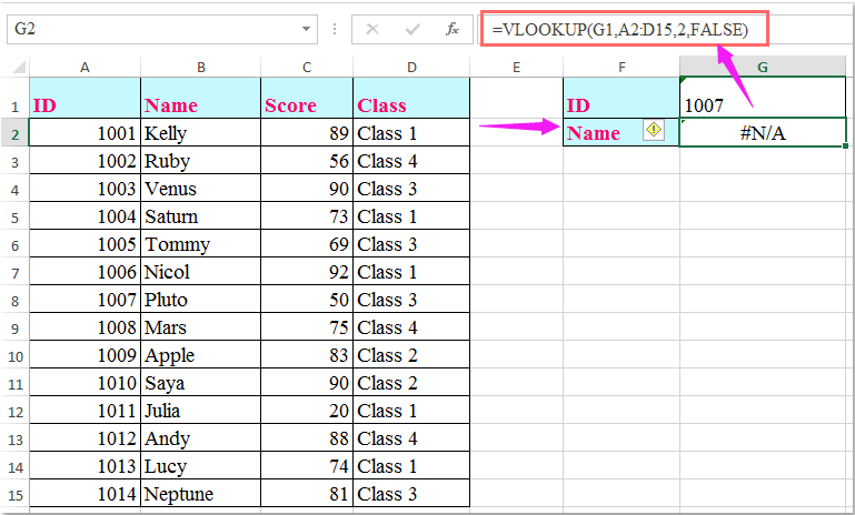
Ag ceapadh, tá an raon sonraí seo a leanas agam, is í an uimhir aitheantais sa tábla bunaidh formáid uimhreach, sa chill amharc a stóráiltear mar théacs, nuair a chuirim an ghnáthfheidhm VLOOKUP i bhfeidhm, gheobhaidh mé toradh earráide mar atá thíos an pictiúr a thaispeántar. Sa chás seo, conas a d’fhéadfainn an fhaisnéis cheart a fháil má tá an fhormáid dhifriúil sonraí ag an uimhir amharc agus an uimhir bhunaidh sa tábla?

Uimhreacha Vlookup stóráilte mar théacs le foirmlí

uimhir vlookup doc stóráilte mar théacs 1


mboilgeog cheart gorm saighead Uimhreacha Vlookup stóráilte mar théacs le foirmlí

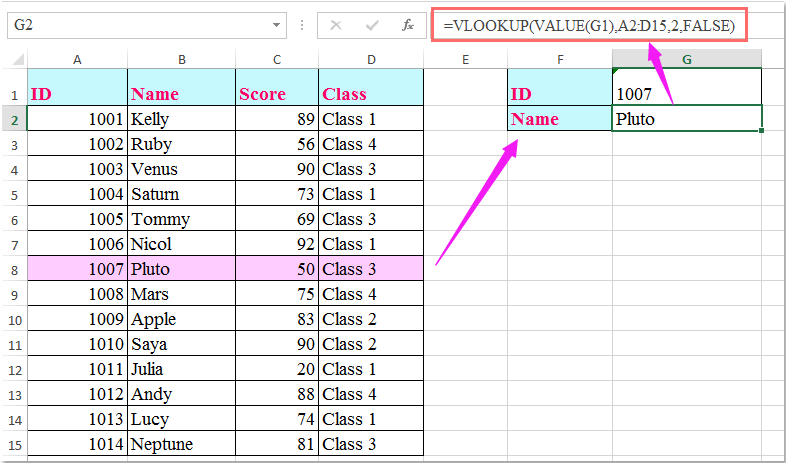
Má tá d’uimhir amharc stóráilte mar théacs, agus an uimhir bhunaidh sa tábla i bhformáid fíoruimhir, cuir an fhoirmle seo a leanas i bhfeidhm chun an toradh ceart a chur ar ais:

Iontráil an fhoirmle seo: = VLOOKUP (LUACH (G1), A2: D15,2, BRÉAGACH) isteach i gcill bhán inar mian leat an toradh a aimsiú, agus brúigh Iontráil eochair chun an fhaisnéis chomhfhreagrach a theastaíonn uait a chur ar ais, féach an scáileán:

uimhir vlookup doc stóráilte mar théacs 2

Nótaí:

1. San fhoirmle thuas: G1 na critéir ar mhaith leat breathnú orthu, A2: D15 an raon tábla ina bhfuil na sonraí a theastaíonn uait a úsáid, agus an uimhir 2 léiríonn sé uimhir an cholúin a bhfuil an luach comhfhreagrach aige a theastaíonn uait a thabhairt ar ais.

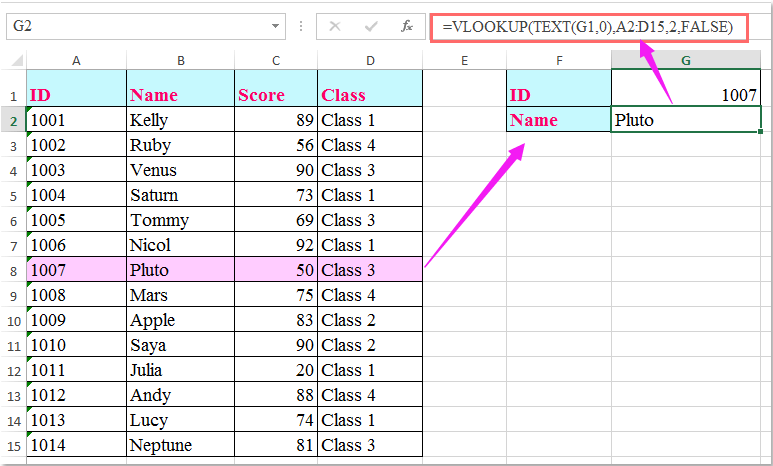
2. Más formáid uimhreach do luach cuardaigh, agus má stóráiltear an uimhir aitheantais sa tábla bunaidh mar théacs, ní oibreoidh an fhoirmle thuas, ba cheart duit an fhoirmle seo a chur i bhfeidhm: = VLOOKUP (TEXT (G1,0), A2: D15,2, BRÉAGACH) chun an toradh ceart a fháil de réir mar is gá duit.

uimhir vlookup doc stóráilte mar théacs 3

3. Mura bhfuil tú cinnte cathain a bheidh uimhreacha agat agus cathain a bheidh téacs agat, is féidir leat an fhoirmle seo a úsáid: =IFERROR(VLOOKUP(VALUE(G1),A2:D15,2,0),VLOOKUP(TEXT(G1,0),A2:D15,2,0)) an dá chás a láimhseáil.

Uirlisí Táirgiúlachta Oifige is Fearr

🤖 Kutools AI Aide: anailís sonraí a réabhlóidiú bunaithe ar: Forghníomhú Chliste   |  Gin Cód  |  Cruthaigh Foirmlí Saincheaptha  |  Anailís a dhéanamh ar Sonraí agus Cairteacha a Ghin  |  Feidhmeanna Kutools a agairt...
Gnéithe Coitianta: Faigh, Aibhsigh nó Aithnigh Dúblaigh   |  Scrios Sraitheanna Bána   |  Comhcheangail Colúin nó Cealla gan Sonraí a Chailleadh   |   Babhta gan Foirmle ...
Cuardaigh Super: Ilchritéir VLookup    VLookup Illuachanna  |   VLookup Trasna Ilbhileoga   |   Amharc doiléir ....
Liosta anuas Casta: Go tapa Cruthaigh Liosta Anuas   |  Liosta anuas Cleithiúnach   |  Liosta Buail Isteach Ilroghnacha ....
Bainisteoir Colún: Cuir Líon Sonrach Colún leis  |  Colúin Bog  |  Scoránaigh Stádas Infheictheachta na gColún Ceilte  |  Déan comparáid idir Raonta & Colúin ...
Gnéithe Réadmhaoin: Fócas Eangaí   |  Amharc Dearaidh   |   Barra Mór na Foirmle    Leabhar Oibre & Bainisteoir Bileog   |  Leabharlann Acmhainní (Uaththéacs)   |  Piocálaí Dáta   |  Comhcheangail Bileoga Oibre   |  Criptigh/Díchriptigh Cealla    Seol Ríomhphost trí Liosta   |  Scagaire Super   |   Scagaire Speisialta (scagaire trom/iodálach/stailc tríd...) ...
Barr 15 Uirlisí12 Téacs uirlisí (Cuir Téacs, Bain Carachtair,...)   |   50 + Cairt cineálacha (Cairt Gantt,...)   |   40+ Praiticiúil Foirmlí (Ríomh aois bunaithe ar lá breithe,...)   |   19 Insertion uirlisí (Cuir isteach Cód QR, Ionsáigh Pictiúr ón gCosán,...)   |   12 Tiontú uirlisí (Uimhreacha le Focail, Comhshó Airgeadra,...)   |   7 Cumaisc & Scoilt uirlisí (Sraitheanna Comhcheangail Casta, Cealla Scoilt,...)   |   ... agus eile

Supercharge Do Scileanna Excel le Kutools le haghaidh Excel, agus Éifeachtúlacht Taithí Cosúil Ná Roimhe. Kutools le haghaidh Excel Tairiscintí Níos mó ná 300 Ardghnéithe chun Táirgiúlacht a Treisiú agus Sábháil Am.  Cliceáil anseo chun an ghné is mó a theastaíonn uait a fháil ...

Tuairisc


Tugann Tab Oifige comhéadan Tabbed chuig Office, agus Déan Do Obair i bhfad Níos Éasca

  • Cumasaigh eagarthóireacht agus léamh tabbed i Word, Excel, PowerPoint, Foilsitheoir, Rochtain, Visio agus Tionscadal.
  • Oscail agus cruthaigh cáipéisí iolracha i gcluaisíní nua den fhuinneog chéanna, seachas i bhfuinneoga nua.
  • Méadaíonn do tháirgiúlacht 50%, agus laghdaíonn sé na céadta cad a tharlaíonn nuair luch duit gach lá!
Comments (13)
No ratings yet. Be the first to rate!
This comment was minimized by the moderator on the site
Worked. Thank you! 
This comment was minimized by the moderator on the site
Hello,
You are welcome. Glad it helps. Any questions, please feel free to contact us. Have a great day.
Sincerely,
Mandy
This comment was minimized by the moderator on the site
Thanks so much!!!!! This worked for me, the #3 solution! HUGE help!!!
This comment was minimized by the moderator on the site
Hello,
You are welcome. Glad it helps. Any questions, please feel free to contact us. Have a great day.
Sincerely,
Mandy
This comment was minimized by the moderator on the site
Thank You... :) Its worked for me
This comment was minimized by the moderator on the site
Hello,
You are welcome. Glad it helps. Any questions, please feel free to contact us. Have a great day.
Sincerely,
Mandy
This comment was minimized by the moderator on the site
Same thing here. The problem is the data range. For some reason, even when the data type is text, MS Excel still looks at it as a number. But if you hit enter, it looks at it as text. So I usually end up with the data range where some of it is numbers and others, text.

SOLUTION: Use IFERROR function to address BOTH possibilities: IFERROR(VLOOKUP(TEXT(A1,0),$A$1:$A$100,1,FALSE),VLOOKUP(VALUE(A1),$A$1:$A$100,1,FALSE)). Hope this helps.
This comment was minimized by the moderator on the site
Unfortunately this method does not Always work. I import numbers in a column defined as tekst. I lookup these numbers in a table in which the numbers are also stored as tekst. I would say a Vlookup should work, but nor the standard lookup, nor the lookup with TEXT() or VALUE() function as expected. When I retype all values in the columns it works as expected, so there's no error in the formula.
This comment was minimized by the moderator on the site
I have the same problem @Rens, does anybody know a solution for this?
This comment was minimized by the moderator on the site
Same thing here. The problem is the data range. For some reason, even when the data type is text, MS Excel still looks at it as a number. But if you hit enter, it looks at it as text. So I usually end up with the data range where some of it is numbers and others, text.

SOLUTION: Use IFERROR function to address BOTH possibilities: IFERROR(VLOOKUP(TEXT(A1,0),$A$1:$A$100,1,FALSE),VLOOKUP(VALUE(A1),$A$1:$A$100,1,FALSE)). Hope this helps.
This comment was minimized by the moderator on the site
This is what I do and is perfect.
This comment was minimized by the moderator on the site
Same thing here. The problem is the data range. For some reason, even when data type is text, it looks like it's still looked on as a number. But if you hit enter, it looks at it as text. So I usually would end up with the data range where some of it is numbers and others text.

SOLUTION: Use IFERROR function to address BOTH possibilities: IFERROR(VLOOKUP(TEXT(A1,0),$A$1:$A$100,1,FALSE),VLOOKUP(VALUE(A1),$A$1:$A$100,1,FALSE)). Hope this helps.
This comment was minimized by the moderator on the site
Hello Jaji, thanks, this works, I hope in all cases. Nevertheless it looks like a bug to me.
There are no comments posted here yet
Please leave your comments in English
Posting as Guest
×
Rate this post:
0   Characters
Suggested Locations