
Conas an chéad luach neamh-nialasach a chuardach agus an ceanntásc colún comhfhreagrach a chur ar ais in Excel?

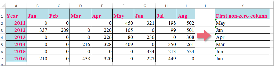
Ag ceapadh, tá raon sonraí agat, anois, ba mhaith leat ceanntásc an cholúin a thabhairt ar ais sa tsraith sin ina dtarlaíonn an chéad luach neamh-nialasach mar a leanas an pictiúr a thaispeántar, an t-alt seo, tabharfaidh mé foirmle úsáideach isteach chun déileáil leis an tasc seo in Excel.

doc lookup an chéad neamh nialas 1

Cuardaigh an chéad luach neamh-nialasach agus seol ceanntásc an cholúin chomhfhreagraigh ar ais leis an bhfoirmle


mboilgeog cheart gorm saighead Cuardaigh an chéad luach neamh-nialasach agus seol ceanntásc an cholúin chomhfhreagraigh ar ais leis an bhfoirmle

Chun ceanntásc an cholúin den chéad luach neamh-nialasach a chur ar ais i ndiaidh a chéile, d’fhéadfadh an fhoirmle seo a leanas cabhrú leat, déan mar seo le do thoil:

Iontráil an fhoirmle seo: =INDEX($B$1:$I$1,MATCH(TRUE,INDEX(B2:I2<>0,),0)) isteach i gcill bhán inar mian leat an toradh a aimsiú, K2, mar shampla, agus ansin tarraing an láimhseáil líonta síos go dtí na cealla ar mhaith leat an fhoirmle seo a chur i bhfeidhm, agus seoltar na ceanntásca colún comhfhreagracha uile den chéad luach neamh-nialasach ar ais mar a thaispeántar ar an scáileán a leanas:

doc lookup an chéad neamh nialas 2

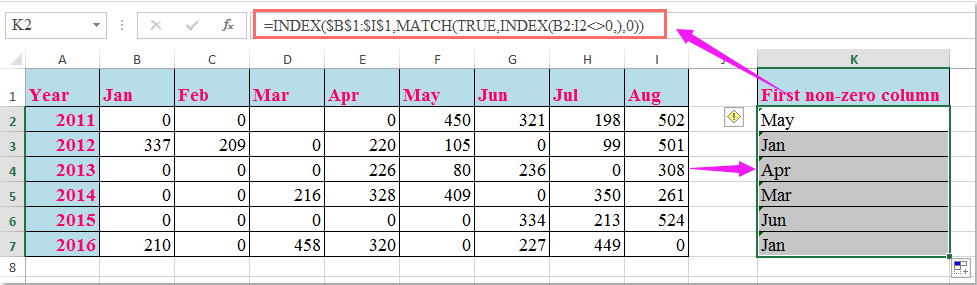
nótaí: San fhoirmle thuas, B1: I1 is é ceanntásca na gcolún is mian leat a thabhairt ar ais, B2: I2 an bhfuil na sonraí as a chéile a theastaíonn uait an chéad luach neamh-nialas a chuardach.

Uirlisí Táirgiúlachta Oifige is Fearr

🤖 Kutools AI Aide: anailís sonraí a réabhlóidiú bunaithe ar: Forghníomhú Chliste   |  Gin Cód  |  Cruthaigh Foirmlí Saincheaptha  |  Anailís a dhéanamh ar Sonraí agus Cairteacha a Ghin  |  Feidhmeanna Kutools a agairt...
Gnéithe Coitianta: Faigh, Aibhsigh nó Aithnigh Dúblaigh   |  Scrios Sraitheanna Bána   |  Comhcheangail Colúin nó Cealla gan Sonraí a Chailleadh   |   Babhta gan Foirmle ...
Cuardaigh Super: Ilchritéir VLookup    VLookup Illuachanna  |   VLookup Trasna Ilbhileoga   |   Amharc doiléir ....
Liosta anuas Casta: Go tapa Cruthaigh Liosta Anuas   |  Liosta anuas Cleithiúnach   |  Liosta Buail Isteach Ilroghnacha ....
Bainisteoir Colún: Cuir Líon Sonrach Colún leis  |  Colúin Bog  |  Scoránaigh Stádas Infheictheachta na gColún Ceilte  |  Déan comparáid idir Raonta & Colúin ...
Gnéithe Réadmhaoin: Fócas Eangaí   |  Amharc Dearaidh   |   Barra Mór na Foirmle    Leabhar Oibre & Bainisteoir Bileog   |  Leabharlann Acmhainní (Uaththéacs)   |  Piocálaí Dáta   |  Comhcheangail Bileoga Oibre   |  Criptigh/Díchriptigh Cealla    Seol Ríomhphost trí Liosta   |  Scagaire Super   |   Scagaire Speisialta (scagaire trom/iodálach/stailc tríd...) ...
Barr 15 Uirlisí12 Téacs uirlisí (Cuir Téacs, Bain Carachtair,...)   |   50 + Cairt cineálacha (Cairt Gantt,...)   |   40+ Praiticiúil Foirmlí (Ríomh aois bunaithe ar lá breithe,...)   |   19 Insertion uirlisí (Cuir isteach Cód QR, Ionsáigh Pictiúr ón gCosán,...)   |   12 Tiontú uirlisí (Uimhreacha le Focail, Comhshó Airgeadra,...)   |   7 Cumaisc & Scoilt uirlisí (Sraitheanna Comhcheangail Casta, Cealla Scoilt,...)   |   ... agus eile

Supercharge Do Scileanna Excel le Kutools le haghaidh Excel, agus Éifeachtúlacht Taithí Cosúil Ná Roimhe. Kutools le haghaidh Excel Tairiscintí Níos mó ná 300 Ardghnéithe chun Táirgiúlacht a Treisiú agus Sábháil Am.  Cliceáil anseo chun an ghné is mó a theastaíonn uait a fháil ...

Tuairisc


Tugann Tab Oifige comhéadan Tabbed chuig Office, agus Déan Do Obair i bhfad Níos Éasca

  • Cumasaigh eagarthóireacht agus léamh tabbed i Word, Excel, PowerPoint, Foilsitheoir, Rochtain, Visio agus Tionscadal.
  • Oscail agus cruthaigh cáipéisí iolracha i gcluaisíní nua den fhuinneog chéanna, seachas i bhfuinneoga nua.
  • Méadaíonn do tháirgiúlacht 50%, agus laghdaíonn sé na céadta cad a tharlaíonn nuair luch duit gach lá!
Comments (15)
No ratings yet. Be the first to rate!
This comment was minimized by the moderator on the site
Hello, my problem is: a have value 1,2,3,4,...50 that are the number of month. How to denormalize month into real datum. Thank you in advance a lot!!!
This comment was minimized by the moderator on the site
Does anyone know what you would do if your cell that contains a zero has a formula in it? When I use this formula, I end up with whatever the first column header is regardless of whether it is zero or not.
This comment was minimized by the moderator on the site
E como faço pra procurar o primeiro valor diferente de zero da esquerda pra direita?
This comment was minimized by the moderator on the site
Hello, Matheus
If you want to return the first non-zero value from a row, please apply the below formula:
=INDEX(B2:F2,MATCH(TRUE,INDEX(B2:F2<>0,),0))
Please have a try, hope it can help you!
This comment was minimized by the moderator on the site
What if you needed the last non-zero value in an array?

P.S. This was really helpful, thank you so much!
This comment was minimized by the moderator on the site
Hello, Ali,
To get the column header based on the last non-zero value, please apply the below formula, see screenshot:
=INDEX($B$1:$H$1,MAX((COLUMN(B2:H2)-MIN(COLUMN(B2:H2))+1)*(B2:H2<>0)))
Please remember to press Ctrl+Shift+Enter key together.
https://www.extendoffice.com/images/stories/comments/comment-skyyang/doc-last-non-zero.png
Please try, hope it can help you!
This comment was minimized by the moderator on the site
The formula is super helpful and helped me sorted out the situation! Thanks!!! Is there any chance you may please help to also explain how it works?
This comment was minimized by the moderator on the site
How do you look up for the second,third and fourth non-zero value?
This comment was minimized by the moderator on the site
Hello, Robert,
To lookup the second, third or fourth non-zero values and return their columns, please apply the below formula: (After pasting the formula, please press Ctr + Shift + Enter keys together.)
=INDEX($B$1:$I$1,SMALL(IF(B2:I2<>0, COLUMN(B2:I2)-COLUMN(A2)),2))


Note: To extract the third or fourth result, you just need to change the number 2 to 3,4 as you need.

Please have a try, hope it can help you!
This comment was minimized by the moderator on the site
CAN U EXPLIAN HOW THIS FORMULA WORKS
This comment was minimized by the moderator on the site
Hello Priya,I am glad to help. I will separate the formula = INDEX($B$1:$I$1,MATCH(TRUE,INDEX(B2:I2<>0,),0)) into 3 parts, and explain the formula to you step by step.
First, let us see the inner-most formula =INDEX(B2:I2<>0,). This formula returns an array of TRUE and FALSE whether the values of range B2:I2 are equal to 0. Please see the screenshot 1, formula =INDEX(B2:I2<>0,) returns {FALSE,FALSE,FALSE,FALSE,TRUE,TRUE,TRUE,TRUE}.
Second, =MATCH(TRUE,INDEX(B2:I2<>0,),0) =MATCH(TRUE, {FALSE,FALSE,FALSE,FALSE,TRUE,TRUE,TRUE,TRUE}, 0). It returns the position of the first value "TRUE", while 0 in the formula means an exact match. We can see that the first value "TRUE" occurs at the 5th position of the array. Then the second formula returns 5. See the screenshot 2.
Finally,  =INDEX(B1:I1,MATCH(TRUE,INDEX(B2:I2<>0,),0))=INDEX(B1:I1,5). It returns the 5th value of the array B1:I1. We can see in the screenshot that the value is "May". So the final formula returns "May". 
PS: To drag the fill handle down the formula to get the rest of the results, we must make the range B1:I1 absolute. So we add $ to range B1:I1 to keep it absolute. 
Hope my explanation can solve your puzzle. Have a nice day.
Sincerely,Mandy
This comment was minimized by the moderator on the site
Thank you Mandy for illustrating it in detail.
Kindly guide how to get the last non zero value from same formula instead of first non zero value.
Will Match work for that or not?
This comment was minimized by the moderator on the site
Hi MandyZhou,

Thank you for the explanation!
I have a follow-up question.
How would the formula change if you had to look up the year too?
So in the above example, let's assume that column J is 'Year' and that in cell J2 is written '2015'.
And in cell K2 I would need the column header for the first non-zero value of the year in L2 (year 2015, so I would need to find 'Jun' in cell K2).

Thanks in advance for your help!
Jason
This comment was minimized by the moderator on the site
How can I return the second and third, etc non zero value? Your formula is amazing but I am trying to search more keywords from a text so sometimes they are 2 or 3 in the same sentence
This comment was minimized by the moderator on the site
se volessi "l'ultimo" Valore Diverso Da Zero E Restituire L'intestazione Della Colonna Corrispondente Con La Formula?
There are no comments posted here yet
Please leave your comments in English
Posting as Guest
×
Rate this post:
0   Characters
Suggested Locations